Kibana is a tool from Elastic that makes analysis of data held in Elasticsearch really easy and very powerful. Because Elasticsearch has very loose schema that can evolve on demand it makes it very quick to get up and running with some cool visualisations and analysis on any set of data. I demonstrated this in a blog post last year, taking a CSV file and loading it into Elasticsearch via Logstash.
This is all great, but the one real sticking point with analytics in Elasticsearch/Kibana is that it needs the data to be denormalised. That is, you can’t give it a bunch of sources of data and it perform the joins for you in Kibana - it just doesn’t work like that. If you’re using Elasticsearch alone for analytics, maybe with a bespoke application, there are ways of approaching it, but not through Kibana. Now, depending on where the data is coming from, this may not be a problem. For example, if you use the JDBC Logstash input to pull from an RDBMS source you can specify a complex SQL query going across multiple tables, so that the data when it hits Elasticsearch is nice and denormalised and ready for fun in Kibana. But, source data doesn’t always come this way, and it’s useful to have a way to work with the data still when it is like this.
I was playing around with some data recently (as one does, of course 8-) ) to try and load Elasticsearch so as to look at the Graph function in more detail, but struggling because the data itself was mostly made of codes that were foreign keys to separate datasets. The data was a CSV from data.gov.uk, detailing road accidents. Each field, such as the police force, was simply a code that then had to be looked up on an Excel document available separately. Loading just the main CSV into Elasticsearch was easy enough (see github for details), but of limited use once in Kibana:

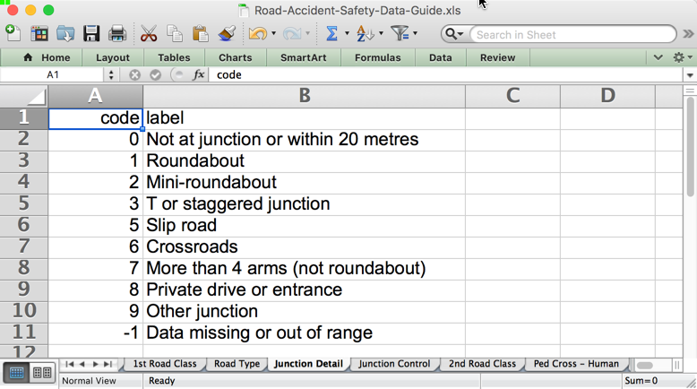
Day_of_Week being from 1 to 7 I could probably hazard a guess at the lookup value myself, but Junction_Detail of “8” … not a clue. To find out, I need to match each foreign key with the corresponding lookup data, which is in a set of sheets in an Excel document:

At this point we are at the official start of “wrangling” the data. We don’t know what we can do with the data until we’ve got it in a structure that makes it useful, so we don’t want to front-load the time needed for discovery with some complex ETL if the data’s not going to turn out to yield much of interest. We could use a data integration tool such as ODI, but talk about sledgehammer to crack a nut … and that’s before we take into account license costs, infrastructure overheard, and so on. Surely we can do this more smartly, as a one-off or hacky-repeatable thing, until we’re sure it’s going to be of worth to ‘productionise’.
First up was trying to keep the toolset down to a minimum, and modifying the CSV file from bash itself. People sometimes forget that bash comes with a fantastically powerful set of data manipulation tools, in the form of sed, awk, tr, grep, and so on. One of these is also join, which as the name says, let’s you take two files and join on a given column. However, after a few iterations (read: bouncing back and forth between the terminal and Google and nearly throwing my laptop at the wall) I wrote it off as unfeasible. Problems with character encoding of the datasets, and the fact that I had to manually extract the data from Excel first before I could run it - not to mention the fact there are nearly 20 dimensions to join - meant that I discounted this option.
I then had one of those “ahhhhh” moments, remembering the excellent work that my colleague Jordan Meyer did at the Rittman Mead BI Forum last year in his Data Discovery and Predictive Modelling masterclass. In it he extolled the many virtues of R for working with data. Not only is R a powerful statistics language, it’s also a damn useful (and, I would say, elegant) one for manipulating data, helped in large part by the dplyr package. It also has lots of libraries for doing useful stuff like reading CSV files based on the headers without having to declare the column, as well as reading natively from Excel files. So, off we go:
### Load main accident facts from CSV
library('readr')
accidents <- read_csv("/tmp/dft/DfTRoadSafety_Accidents_2014.csv")
N.B. If you’ve any libraries here not already installed, you can install using install.packages('foo')
With the data loaded, let’s now set a proper timestamp column, since in the data there’s only Date and Time on their own. We can see some sample values with the head function:
> head(accidents$Date)
[1] "09/01/2014" "20/01/2014" "21/01/2014" "15/01/2014" "09/01/2014"
[6] "17/01/2014"
> head(accidents$Time)
[1] "13:21" "23:00" "10:40" "17:45" "08:50" "14:11"
>
Handling and parsing dates is a problem to be solved across all languages and technologies, and R’s lubridate package is by far the best way I’ve ever seen. Using lubridate you describe the order that the date/time components appear in (e.g. “year month day”) but without needing to specify the exact format string usually needed, thus avoiding the usual monkeying around with letter symbols, counting out the right number of them and getting the case right (is it YYYYMMDD or YYYYmmDD or YYMD?). In the above data sample you can see that the date is in the form Day / Month / Year, and the Time is Hour / Minute. That’s all we need to know - forget having to check if “MM” is month or minute, whether to escape the separators and so on. Since it’s Day / Month / Year / Hour / Minute, we use the dmy_hm function:
### Populate a timestamp using the awesome lubridate package
library('lubridate')
### Using "dmy_hm" we're telling lubridate that the date is in the order
### Day / Month / Year / Hour / Minute - the actual format string and
### separators get figured out automagically
accidents$timestamp <- dmy_hm(paste(accidents$Date,accidents$Time))
The data includes the geo-spatial reference points, which Elasticsearch can store enabling analysis of the data in tools including Kibana. To store this properly we define location as a geo_point in the mapping, and concatenate the latitude and longitude:
### Define the location as a string.
accidents$location <- paste(accidents$Latitude,accidents$Longitude,sep=',')
At this point we have just our main “fact” dataset, including properly formatted and typed Timestamp column:
> str(accidents)
Classes 'tbl_df', 'tbl' and 'data.frame':	146322 obs. of  33 variables:
 $ Accident_Index                             : chr  "201401BS70001" "201401BS70002" "201401BS70003" "201401BS70004" ...
 $ Location_Easting_OSGR                      : int  524600 525780 526880 525580 527040 524750 524950 523850 524500 526450 ...
 $ Location_Northing_OSGR                     : int  179020 178290 178430 179080 179030 178970 179240 181450 180260 179230 ...
 $ Longitude                                  : num  -0.206 -0.19 -0.174 -0.192 -0.171 ...
 $ Latitude                                   : num  51.5 51.5 51.5 51.5 51.5 ...
 $ Police_Force                               : int  1 1 1 1 1 1 1 1 1 1 ...
 $ Accident_Severity                          : int  3 3 3 3 3 3 3 3 3 3 ...
> head(accidents$timestamp)
[1] "2014-01-09 13:21:00 UTC" "2014-01-20 23:00:00 UTC"
[3] "2014-01-21 10:40:00 UTC" "2014-01-15 17:45:00 UTC"
[5] "2014-01-09 08:50:00 UTC" "2014-01-17 14:11:00 UTC"
>
Now let’s load a lookup dataset for one of the dimensions – Police Force.
library('readxl')
police <-
  read_excel("/tmp/dft/Road-Accident-Safety-Data-Guide.xls",sheet = 3)
We can check the data:
> library('tibble')
> as_data_frame(police)
Source: local data frame [51 x 2]

    code               label
   <dbl>               <chr>
1      1 Metropolitan Police
2      3             Cumbria
3      4          Lancashire
4      5          Merseyside
[...]
but note the second column heading – label. When we come to do our joining we want the name of this descriptor column to reference the dimension to which it is attached. So, we rename it using a function in the dplyr library:
> library('dplyr')
> police <-
   police %>%
   rename(police_force=label)
> as_data_frame(police)
Source: local data frame [51 x 2]

    code        police_force
   <dbl>               <chr>
1      1 Metropolitan Police
2      3             Cumbria
3      4          Lancashire
4      5          Merseyside
[...]
Much better! Now to join this to the main dataset. For this we use dplyr again, with its join function:
accidents <-
  left_join(accidents,police, by=c("Police_Force"="code"))
If you want to see more about working with R, there’s a great reference PDF here: Data Wrangling with dplyr and tidyr Cheat Sheet.
Check out the results:
> accidents %>%
+ select(1,34)
Source: local data frame [146,322 x 2]

   Accident_Index        police_force
            <chr>               <chr>
1   201401BS70001 Metropolitan Police
2   201401BS70002 Metropolitan Police
3   201401BS70003 Metropolitan Police
Once the joining is done it’s off to another R library, this time elastic, enabling us to write the denormalised data frame directly into Elasticsearch. We’re manually defining Accident_Index as the unique key for the record, so that if re-run Elasticsearch won’t accept duplicate entries.
library("elastic")
### connect() assumes Elasticsearch is running locally on port 9200
connect()
docs_bulk(accidents,doc_ids = accidents$Accident_Index,index="dftroadsafetyaccidents02")
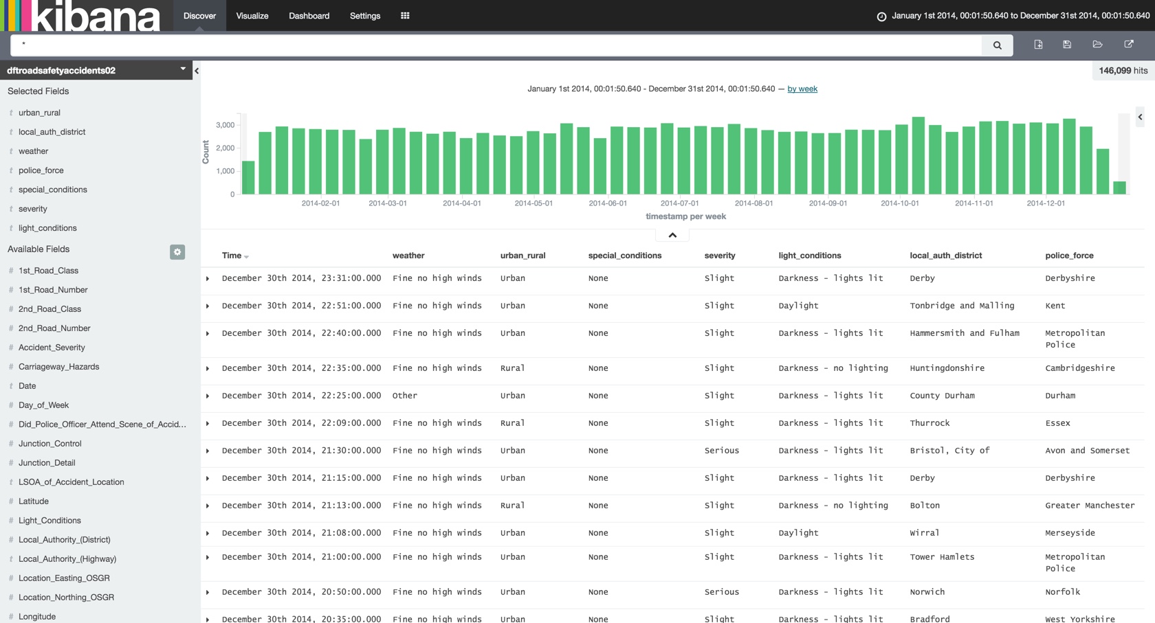
Heading over to Kibana we now have the basis from which to start usefully exploring the data …

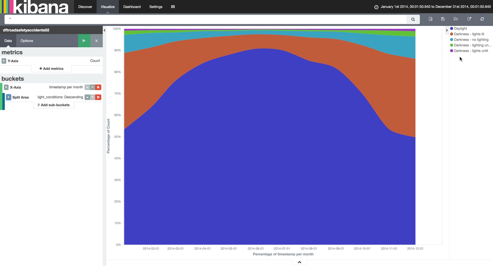
… as well as knocking out aggregate visualisations with ease:

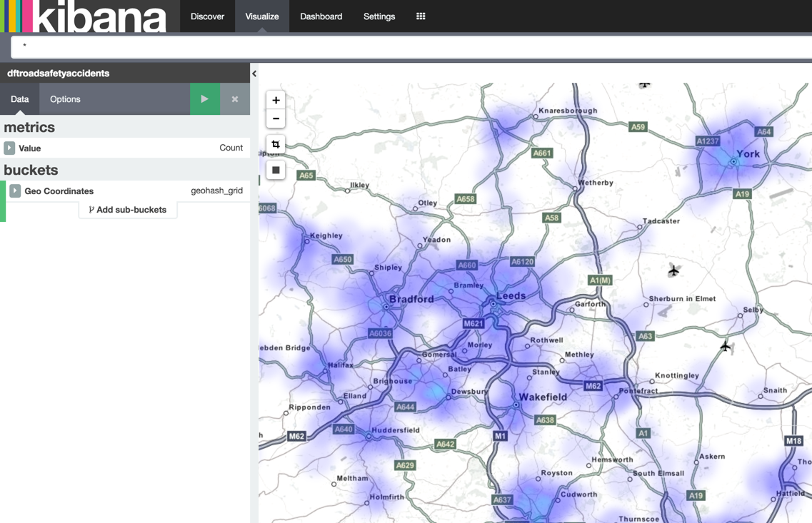
And since we stored the data using the geo-spatial reference format we can also map it out:

Stay tuned for more details of the actual Graph analysis that I did with the data once it was loaded….
You can find the full R code on github here, including joins to all 18 lookup data sets. There’s also the code for loading the data into Elasticsearch directly via Logstash from the CSV, and the necessary Elasticsearch mapping template.
