In this blog post I’m going to explore how as a data engineer in the field today I might go about putting together a rudimentary data pipeline. I’ll take some operational data, and wrangle it into a form that makes it easily pliable for analytics work.
After a somewhat fevered and nightmarish period during which people walked around declaring "Schema on Read" was the future, that "Data is the new oil", and "Look at the size of my big data", the path that is history in IT is somewhat coming back on itself to a more sensible approach to things.
As they say:
What’s old is new
This is good news for me, because I am old and what I knew then is 'new' now ;)
Overview 🔗
The Data 🔗
| this uses Environment Agency flood and river level data from the real-time data API (Beta) |
If you’ve been following this blog closely you’ll have seen some of my noodlings around with this data already. I wrote about exploring it with DuckDB and Rill, using it as an excuse to try out the new DuckDB UI, as well as loading it into Kafka and figuring out what working with it in Flink SQL would look like.
At the heart of the data are readings, providing information about measures such as rainfall and river levels. These are reported from a variety of stations around the UK.

The data is available on a public REST API (try it out here to see the current river level at one of the stations in Sheffield).
The Plan 🔗

I’m going to make heavy use of DuckDB for this project. It can read data from REST APIs, it can process data, and it can store data. What’s more, it can be queried with various visualisation tools including Rill Data, Superset, and Metabase, as we’ll see later.
Once loaded, the dimension data will be brute-force rebuilt based on the latest values. For those who like this kind of thing (and who doesn’t), this is in effect Slowly-Changing Dimension (SCD) type 1. With SCD Type 1, no history is retained. This means that if a measure or station is removed, associated readings previously recorded will not have a match on the corresponding dimension table. If it’s updated, historical readings will be shown with the dimension data as-is now, not as-was then.
The readings fact data we’ll collect in a fact table that will mostly be appended to with each incremental load.
It’s not entirely that simple though:
-
Some stations may lag in reporting their data, so we might pull duplicates (i.e. the reading for the last time period when it did report)
-
Some stations may batch their reporting, so we need to handle polling back over a period of time and dealing with the resulting duplicates for readings that had been reported
In addition, historical data is available and we want to be able to include that too.
Once we’ve got our fact and dimension data sorted, we’ll join it into a denormalised table that we can build analytics against.
The Environment 🔗
I’m running this all locally on my Mac. The first step is to install DuckDB and a few other useful tools:
brew install duckdb httpie jqThen fire up DuckDB with its notebook-like UI (you don’t have to use the UI; you can use whatever interface you want):
duckdb env-agency.duckdb -uiExtract (with just a little bit of transform) 🔗
The basic ingest looks like this:
CREATE OR REPLACE TABLE readings_stg AS
    SELECT * FROM read_json('https://environment.data.gov.uk/flood-monitoring/data/readings?latest')
DuckDB automagically determines the schema of the table. We’re going to do one bit of processing at this stage too.
By default all the API calls return a payload made up of metadata and then an array of the actual data. I decided to explode out the array at this point of ingest just to make things a bit easier.
At this point I’m throwing away the @context and meta data elements; you may decide you want to keep them.
|
CREATE OR REPLACE TABLE readings_stg AS
  WITH src AS (SELECT *
                FROM read_json('https://environment.data.gov.uk/flood-monitoring/data/readings?latest'))
    SELECT u.* FROM (
        SELECT UNNEST(items) AS u FROM src);

CREATE OR REPLACE TABLE measures_stg AS
  WITH src AS (SELECT *
                FROM read_json('https://environment.data.gov.uk/flood-monitoring/id/measures'))
    SELECT u.* FROM (
        SELECT UNNEST(items) AS u FROM src);

CREATE OR REPLACE TABLE stations_stg AS
  WITH src AS (SELECT *
                FROM read_json('https://environment.data.gov.uk/flood-monitoring/id/stations'))
    SELECT u.* FROM (
        SELECT UNNEST(items) AS u FROM src);
Let’s see what data we’ve pulled in:
SELECT 'readings_stg' AS table_name, COUNT(*) as row_ct, min(dateTime) as min_dateTime, max(dateTime) as max_dateTime FROM readings_stg
UNION ALL
SELECT 'measures_stg' AS table_name, COUNT(*) as row_ct,NULL,NULL from measures_stg
UNION ALL
SELECT 'stations_stg' AS table_name, COUNT(*) ,NULL,NULL from stations_stg;
table_name row_ct min_dateTime max_dateTime
readings_stg 5272 2025-02-21 13:45:00 2025-03-20 13:25:10
measures_stg 6638
stations_stg 5400The latest dateTime value looks right (it’s 2025-03-20 13:42:45 as I write this) but why is the minimum nearly a month ago?
This is where the DuckDB UI’s data viz comes in useful:
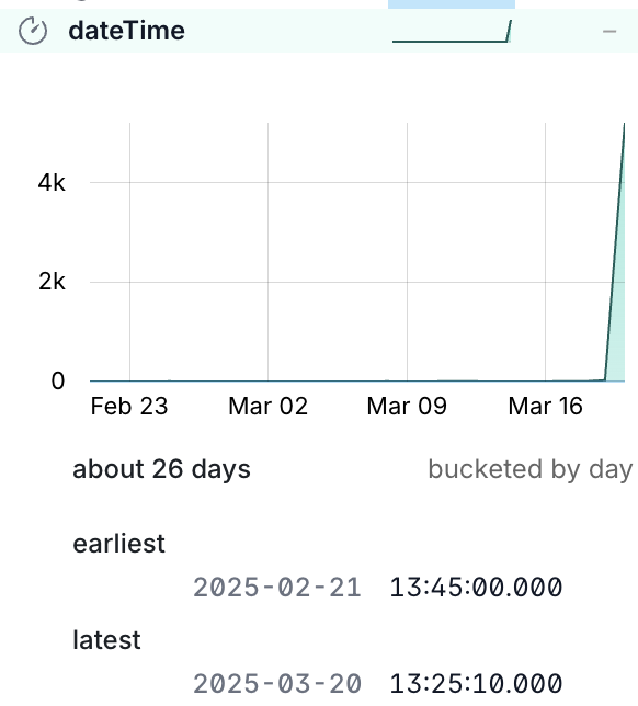
What this shows us is that almost all the data is for the latest timestamp, with just a handful of readings for other dates.
We can prove this out with a SQL query too:
SELECT dateTime, COUNT(*) AS reading_count
    FROM readings_stg
    GROUP BY dateTime
    ORDER BY 2 desc, 1 desc;
Transform 🔗
Keys 🔗
The staging tables have no keys defined, because YOLO right? Well no. Staging is where we bring in the source data, warts and all. A station shouldn’t have more than one instance, but who says that’s the case?
Rather than failing the ingest because of a logical data error, it’s our job to work with what we’ve got. That means coding defensively and ensuring that whilst we’ll accept anything into the staging area, we don’t blindly propagate crap through the rest of the pipeline.
One of the ways to enforce this is constraints, of which primary keys are an example.

Readings→Measures 🔗
Unchanged, the data in readings relates to measures on the readings.measure column:
http://environment.data.gov.uk/flood-monitoring/id/measures/5312TH-level-stage-i-15_min-mASDOn measures the @id column matches this:
http://environment.data.gov.uk/flood-monitoring/id/measures/5312TH-level-stage-i-15_min-mASDBut this is duplicated in the notation column, minus the http://environment.data.gov.uk/flood-monitoring/id/measures/ URL prefix:
5312TH-level-stage-i-15_min-mASDWe’ll pre-process the readings.measure column to strip this prefix to make the join easier (and simpler to debug, since you’re not wading through columns of long text).
Measures→Stations 🔗
The station for which a reading was taken is found via the measure, since measures are unique to a station.
On measures the station column is the foreign key:
http://environment.data.gov.uk/flood-monitoring/id/stations/SP50_72Again, the URL prefix (http://environment.data.gov.uk/flood-monitoring/id/stations/) is repeated and we’ll strip that out.
One thing that caught me out here is that the station (minus the URL prefix) and the stationReference are almost always the same.
Almost always.
I spent a bunch of time chasing down duplicates after the subsequent join to the fact table resulted in a fan-out, because stationReference isn’t unique.
SELECT stationReference, station
    FROM measures
    WHERE station!=stationReference
    ORDER BY stationReference;
stationReference station
4063TH 4063TH-southern
4063TH 4063TH-thames
E22300 E22300-anglian
E22300 E22300-southern
E22300 E22300-southern
[…]26 rows out of 6612…enough to cause plenty of trouble when I made assumptions about the data I was eyeballing and missed the 0.4% exceptions…
It does state it clearly in the API doc; station is the foreign key, not stationReference.
RTFM, always ;)
Dimension tables 🔗
Building the dimension tables is simple, if crude, enough.
With a CREATE OR REPLACE we tell DuckDB to go ahead and create the table, and if it exists already, nuke it and create a fresh version.
The transformation we’ll do is pretty light.
Measures 🔗
We’re going to drop a couple of fields:
-
@idwe don’t need -
latestReadingholds fact data that we’re getting from elsewhere, so no point duplicating it here
We’ll also transform the foreign key to strip the URL prefix making it easier to work with.
CREATE OR REPLACE TABLE measures AS
    SELECT *
            EXCLUDE ("@id", latestReading)
            REPLACE(
                REGEXP_REPLACE(station,
                        'http://environment\.data\.gov\.uk/flood-monitoring/id/stations/',
                        '') AS station
            )
    FROM measures_stg;
This is using a couple of my favourite recent discoveries in DuckDB—the EXCLUDE and REPLACE clauses.
With EXCLUDE we’re taking advantage of SELECT * to bring in all columns from the source table—which saves typing, but also means new columns added to the source will propagate automagically—but with the exception of ones that we don’t want.
The REPLACE clause is a really elegant way of providing a different version of the same column.
Since we want to retain the station column but just trim the prefix, this is a great way to do it without moving its position in the column list.
The other option would have been to EXCLUDE it too, and then add it on to the column list.
With the table created let’s define the primary key as discussion above:
ALTER TABLE measures
    ADD CONSTRAINT measures_pk PRIMARY KEY (notation);
Stations 🔗
Very similar to the process above:
CREATE OR REPLACE TABLE stations AS
    SELECT * EXCLUDE (measures)
    FROM stations_stg;

ALTER TABLE stations
    ADD CONSTRAINT stations_pk PRIMARY KEY (notation);
One thing that you might also do is move the primary key (notation) to be the first column in the table.
This is a habit I picked up years ago; I don’t know if it’s still common practice.
To do it you’d EXCLUDE the field and manually prefix it to the star expression:
CREATE OR REPLACE TABLE stations AS
    SELECT notation, * EXCLUDE (measures, notation)
    FROM stations_stg;

ALTER TABLE stations ADD CONSTRAINT stations_pk PRIMARY KEY (notation);
(If you do this, you’d want to logically do the same for the other tables' PKs too).
Fact table 🔗
This is where things get fun :)
Because we’re going to be adding to the table with new data rather than replacing it, we can’t just CREATE OR REPLACE it each time.
Therefore we’ll run the CREATE as a one-off:
CREATE TABLE IF NOT EXISTS readings AS
    SELECT * EXCLUDE "@id" FROM readings_stg WHERE FALSE;
A few notes:
-
IF NOT EXISTSmakes sure we don’t overwrite the table. We’d get the same effect if we just putCREATE TABLE, the only difference is the latter would fail if the table already exists, whilstIF NOT EXISTScauses it to exit silently. -
We’re going to
EXCLUDEthe@idcolumn because we don’t need it -
This will only create the table using the schema projected by the
SELECT; theWHERE FALSEmeans no rows will be selected. This is so that we decouple the table creation from its population.
Now we’ll add a primary key.
The key here is the time of the reading (dateTime) plus the measure (measure).
ALTER TABLE readings
    ADD CONSTRAINT readings_pk PRIMARY KEY (dateTime, measure);
Populating the fact table 🔗
Our logic here is: "Add data if it’s new, don’t throw an error if it already exists". Our primary key for this is the time of the reading and the measure. If we receive a duplicate we’re going to ignore it.
We’re making a design choice here; in theory we could decide that a duplicate reading represents an update to the original (re-stating a fact that could have been wrong previously) and handle it as an UPSERT (i.e. INSERT if new, UPDATE if existing).
|
DuckDB has some very nice syntax available around the INSERT INTO … SELECT FROM pattern. To achieve what we want we use the self-documenting statement INSERT OR IGNORE. This is a condensed version of the more verbose INSERT INTO… SELECT FROM… ON CONFLICT DO NOTHING syntax.
INSERT OR IGNORE INTO readings
SELECT *
        EXCLUDE "@id"
        REPLACE(
            REGEXP_REPLACE(measure,
            'http://environment\.data\.gov\.uk/flood-monitoring/id/measures/',
            '') AS measure)
FROM readings_stg
We’re using the same EXCLUDE and REPLACE expressions as we did above; remove the @id column, and strip the URL prefix from the foreign key measure.
The first time we run this we can see the number of INSERTS:
changes: 5272Then we re-run it:
changes: 0Since nothing changed in the staging table, this makes sense. Let’s load the staging table with the latest data again:
changes: 4031Joining the data 🔗
Similar to the fact table above, we’re going to be incrementally loading this final, denormalised, table. I’m taking a slightly roundabout tack to do this here.
First, I’ve defined a view which is the result of the join:
CREATE OR REPLACE VIEW vw_readings_enriched AS
    SELECT  "r_\0": COLUMNS(r.*),
            "m_\0": COLUMNS(m.*),
            "s_\0": COLUMNS(s.*)
            FROM
            readings r
            LEFT JOIN measures m ON r.measure = m.notation
            LEFT JOIN stations s ON m.station = s.notation
See my earlier blog post if you’re not familiar with the COLUMNS syntax
|
From the view I create the table’s schema (but don’t populate anything yet):
CREATE TABLE IF NOT EXISTS readings_enriched AS
    SELECT * FROM vw_readings_enriched LIMIT 0;

ALTER TABLE readings_enriched
    ADD CONSTRAINT readings_enriched_pk PRIMARY KEY (r_dateTime, r_measure);
And now populate it in the same way as we did for the readings table:
INSERT OR IGNORE INTO readings_enriched
    SELECT * FROM vw_readings_enriched;
Query the joined data 🔗
Now that we’ve got our joined data we can start to query and analyse it. Here’s the five most recent readings for all water level measurements on the River Wharfe:
SELECT r_dateTime
		, s_label
		, r_value
FROM readings_enriched
WHERE s_rivername= 'River Wharfe' and m_parameterName = 'Water Level'
ORDER BY r_dateTime desc LIMIT 5 ;
┌─────────────────────┬──────────────────────────────────────┬─────────┐
│ r_dateTime │ s_label │ r_value │
│ timestamp │ json │ double │
├─────────────────────┼──────────────────────────────────────┼─────────┤
│ 2025-03-19 15:00:00 │ "Kettlewell" │ 0.171 │
│ 2025-03-19 15:00:00 │ "Cock Beck Sluices" │ 3.598 │
│ 2025-03-19 15:00:00 │ "Nun Appleton Fleet Pumping Station" │ 2.379 │
│ 2025-03-19 15:00:00 │ "Tadcaster" │ 0.227 │
│ 2025-03-19 15:00:00 │ "Netherside Hall" │ 0.319 │
└─────────────────────┴──────────────────────────────────────┴─────────┘Historical data 🔗
The readings API includes the option for specifying a date range.
However, there is a hard limit of 10000 rows, and a single time period’s readings for all stations is about 5000 rows, this doesn’t look like a viable option if we’re wanting to backfill data for all stations.
Historic readings are available, although in CSV format rather than the JSON we’re used to. Nothing like real-world data engineering problems to keep us on our feet :)
$ http https://environment.data.gov.uk/flood-monitoring/archive/readings-2025-03-18.csv |head -n2
dateTime,measure,value
2025-03-18T00:00:00Z,http://environment.data.gov.uk/flood-monitoring/id/measures/531166-level-downstage-i-15_min-mAOD,49.362
Fortunately, DuckDB has us covered, and handles it in its stride:
🟡◗ SELECT * FROM 'https://environment.data.gov.uk/flood-monitoring/archive/readings-2025-03-18.csv' LIMIT 1;
┌─────────────────────┬──────────────────────────────────────────────────────────────────────────────────────────────────┬─────────┐
│      dateTime       │                                             measure                                              │  value  │
│      timestamp      │                                             varchar                                              │ varchar │
├─────────────────────┼──────────────────────────────────────────────────────────────────────────────────────────────────┼─────────┤
│ 2025-03-18 00:00:00 │ http://environment.data.gov.uk/flood-monitoring/id/measures/531166-level-downstage-i-15_min-mAOD │ 49.362  │
└─────────────────────┴──────────────────────────────────────────────────────────────────────────────────────────────────┴─────────┘
…or almost in its stride—once I ran it on a full file I got this:
CSV Error on Line: 388909
Original Line:
2025-03-17T22:30:00Z,http://environment.data.gov.uk/flood-monitoring/id/measures/690552-level-stage-i-15_min-m,0.770|0.688
Error when converting column "value". Could not convert string "0.770|0.688" to 'DOUBLE'

Column value is being converted as type DOUBLE
This type was auto-detected from the CSV file.
[…]
Bravo for such a verbose and useful error message. Not just "there’s an error", or "could not convert", but tells you where, shows you the line, makes it super-easy to understand the problem and what to do.
What to do? Brush it under the carpet and pretend it didn’t happen!
In other words, ignore_errors=true:
CREATE OR REPLACE TABLE readings_historical AS
  SELECT *
    FROM read_csv('https://environment.data.gov.uk/flood-monitoring/archive/readings-2025-03-18.csv',
                    ignore_errors=true)
This loads all 476k rows of data for 18th March into a new table. Now we’ll add the previous days too—and head out to the shell to do it:
❯ duckdb env-agency.duckdb -c "INSERT INTO readings_historical SELECT * FROM read_csv('https://environment.data.gov.uk/flood-monitoring/archive/readings-2025-03-16.csv', ignore_errors=true);"
100% ▕████████████████████████████████████████████████████████████▏
Run Time (s): real 16.405 user 1.090767 sys 0.516826
Even more concise is the COPY option:
duckdb env-agency.duckdb -c "COPY readings_historical FROM 'https://environment.data.gov.uk/flood-monitoring/archive/readings-2025-03-14.csv' (IGNORE_ERRORS);"
Run Time (s): real 3.275 user 1.718801 sys 0.247875
Why am I doing this from the shell? So that I can then do this:
start_date="2025-01-01"
end_date="2025-03-13"

current_date=$start_date
while [[ "$current_date" < "$end_date" || "$current_date" == "$end_date" ]]; do
    echo "Processing $current_date..."
    duckdb env-agency.duckdb -c \
        "COPY readings_historical
        FROM 'https://environment.data.gov.uk/flood-monitoring/archive/readings-$current_date.csv'
        (IGNORE_ERRORS);"
    current_date=$(date -d "$current_date + 1 day" +%Y-%m-%d)
done
In the readings_historical table is now a nice big chunk of data (not Big Data, just a big chunk of normally-size data):
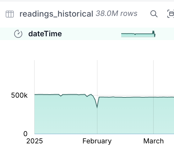
Now to merge this into the main table:
🟡◗ INSERT OR IGNORE INTO readings
    SELECT *
            REPLACE(
                REGEXP_REPLACE(measure,
                'http://environment\.data\.gov\.uk/flood-monitoring/id/measures/',
                '') AS measure)
    FROM readings_historical;
Run Time (s): real 0.003 user 0.002708 sys 0.000571
Conversion Error:
Could not convert string '0.772|0.692' to DOUBLE
Here’s the problem with taking the easy route. By letting DuckDB guess at the data types for the CSV data, we’ve ended up with dodgy data being ingested. How much dodgy data? 0.01%…
🟡◗ SELECT COUNT(*) FROM readings_historical WHERE TRY_CAST(value AS DOUBLE) IS NULL ;┌──────────────┐
│ count_star() │
│ int64 │
├──────────────┤
│ 3202 │
└──────────────┘It took a few minutes to load the historical data, so instead of ditching the table let’s just deal with what we’ve got. First up, what is the dodgy data?
🟡◗ SELECT value
    FROM readings_historical
    WHERE TRY_CAST(value AS DOUBLE) IS NULL
    USING SAMPLE 0.5%;
┌─────────────┐
│ value │
│ varchar │
├─────────────┤
│ 2.415|2.473 │
│ 1.496|1.489 │
│ 1.730|1.732 │
│ 1.419|1.413 │
│ 1.587|1.586 │
│ 1.097|1.101 │
│ 1.032|1.033 │
│ 0.866|0.874 │
│ 0.864|0.862 │
│ 0.861|0.862 │
│ 0.386|0.387 │
│ 1.118|1.062 │
├─────────────┤
│ 12 rows │
└─────────────┘It looks like they all follow this pattern of two valid-looking values separated by a pipe |.
We can double-check this:
🟡◗ SELECT * FROM readings_historical
    WHERE value NOT LIKE '%|%'
    AND TRY_CAST(value AS DOUBLE) IS NULL;
┌───────────┬─────────┬─────────┐
│ dateTime │ measure │ value │
│ timestamp │ varchar │ varchar │
├───────────┴─────────┴─────────┤
│ 0 rows │
└───────────────────────────────┘We’ll make an executive decision to take the first value in these pairs, using REPLACE to override the value to split out the string and use the first instance.
INSERT OR IGNORE INTO readings
    SELECT *
            REPLACE(
                REGEXP_REPLACE(measure,
                'http://environment\.data\.gov\.uk/flood-monitoring/id/measures/',
                '') AS measure,
                SPLIT_PART(value, '|', 1) AS value)
    FROM readings_historical
    WHERE value LIKE '%|%';
Now we can load the rest of the data:
🟡◗ INSERT OR IGNORE INTO readings
        SELECT *
                REPLACE(
                    REGEXP_REPLACE(measure,
                    'http://environment\.data\.gov\.uk/flood-monitoring/id/measures/',
                    '') AS measure)
        FROM readings_historical
        WHERE value NOT LIKE '%|%';
100% ▕████████████████████████████████████████████████████████████▏
Run Time (s): real 218.189 user 213.713807 sys 3.481680
changes: 37031770   total_changes: 37034972
The data’s loaded:
🟡◗ SELECT COUNT(*) as row_ct,
            min(dateTime) as min_dateTime,
            max(dateTime) as max_dateTime
    FROM readings;
┌──────────┬─────────────────────┬─────────────────────┐
│ row_ct │ min_dateTime │ max_dateTime │
│ int64 │ timestamp │ timestamp │
├──────────┼─────────────────────┼─────────────────────┤
│ 37044275 │ 2025-01-01 00:00:00 │ 2025-03-20 15:25:10 │
└──────────┴─────────────────────┴─────────────────────┘Now to load it into the denormalised table—for this it’s the same query as when we’re just loading incremental changes:
INSERT OR IGNORE INTO readings_enriched
    SELECT * FROM vw_readings_enriched;
Let’s "Operationalise" it 🔗
Let’s have a look at a very rough way of running the update for this pipeline automatically.
We’ll create a SQL script to update the dimension data:
-- Load the staging data from the REST API
CREATE OR REPLACE TABLE measures_stg AS
  WITH src AS (SELECT *
                FROM read_json('https://environment.data.gov.uk/flood-monitoring/id/measures'))
    SELECT u.* FROM (
        SELECT UNNEST(items) AS u FROM src);

CREATE OR REPLACE TABLE stations_stg AS
  WITH src AS (SELECT *
                FROM read_json('https://environment.data.gov.uk/flood-monitoring/id/stations'))
    SELECT u.* FROM (
        SELECT UNNEST(items) AS u FROM src);

-- Rebuild dimension tables
CREATE OR REPLACE TABLE measures AS
    SELECT *
            EXCLUDE ("@id", latestReading)
            REPLACE(
                REGEXP_REPLACE(station,
                        'http://environment\.data\.gov\.uk/flood-monitoring/id/stations/',
                        '') AS station
            )
    FROM measures_stg;
ALTER TABLE measures
    ADD CONSTRAINT measures_pk PRIMARY KEY (notation);

CREATE OR REPLACE TABLE stations AS
    SELECT * EXCLUDE (measures)
    FROM stations_stg;

ALTER TABLE stations
    ADD CONSTRAINT stations_pk PRIMARY KEY (notation);
and load the fact data:
-- Load the staging data from the REST API
CREATE OR REPLACE TABLE readings_stg AS
  WITH src AS (SELECT *
                FROM read_json('https://environment.data.gov.uk/flood-monitoring/data/readings?latest'))
    SELECT u.* FROM (
        SELECT UNNEST(items) AS u FROM src);

-- Merge into the fact table
INSERT OR IGNORE INTO readings
SELECT *
        EXCLUDE "@id"
        REPLACE(
            REGEXP_REPLACE(measure,
            'http://environment\.data\.gov\.uk/flood-monitoring/id/measures/',
            '') AS measure)
FROM readings_stg

-- Merge into the denormalised table
INSERT OR IGNORE INTO readings_enriched
    SELECT * FROM vw_readings_enriched;
Now to schedule it.
An entire industry has been built around workflow scheduling tools;
I’m going to stick to the humble cron.
It’s simple, it’s quick, and LLMs have now learnt how to write the syntax ;)
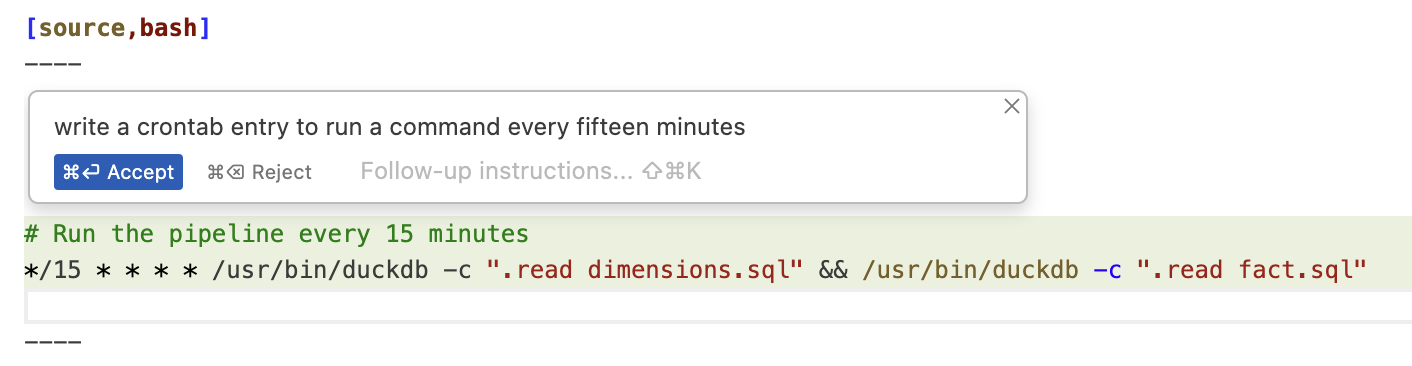
Well, the syntax to invoke DuckDB is a bit different from what Claude thought, but the fiddly */15 stuff it nailed.
Here’s the crontab I set up (crontab -e)
# Run the pipeline every 15 minutes
*/15 * * * * cd ~/env-agency/ && /opt/homebrew/bin/duckdb env-agency.duckdb -f dimensions.sql && /opt/homebrew/bin/duckdb env-agency.duckdb -f fact.sql
Every fifteen minutes this pulls down the latest data, rebuilds the dimension tables, and adds the new data to the fact table.
Analysing the data 🔗
Let’s finish off by looking at how we can analyse the data.
Metabase 🔗
Metabase is fairly quick to get up and running. The complication is that to query DuckDB you need a driver that Motherduck have created that I couldn’t get to work under Docker, hence running Metabase locally:
# You need Java 21
sdk install java 21.0.6-tem

# Download Metabase & Metaduck
mkdir metabase
curl https://downloads.metabase.com/v0.53.7/metabase.jar -O
mkdir plugins && pushd plugins && curl https://github.com/motherduckdb/metabase_duckdb_driver/releases/download/0.2.12-b/duckdb.metabase-driver.jar -O && popd

# Run metabase
java --add-opens java.base/java.nio=ALL-UNNAMED -jar metabase.jar
This launches Metabase on http://localhost:3000, and after an annoying on-boarding survey, it’s remarkably quick to get something created. Adding the database is simple enough:
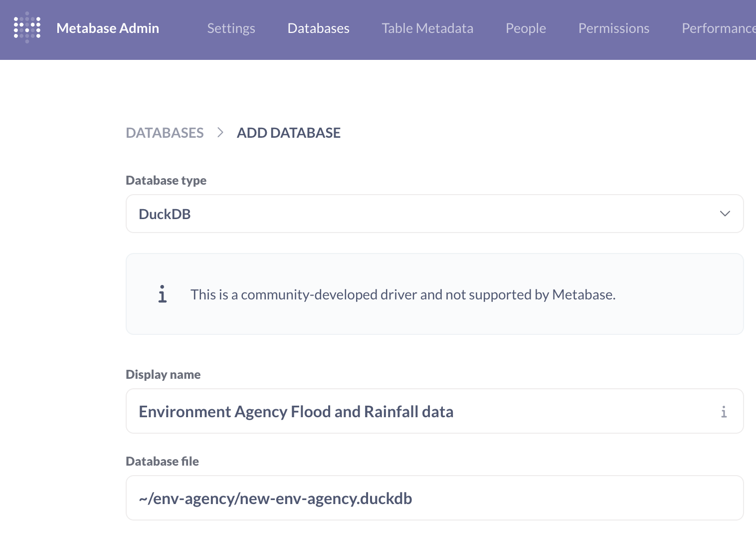
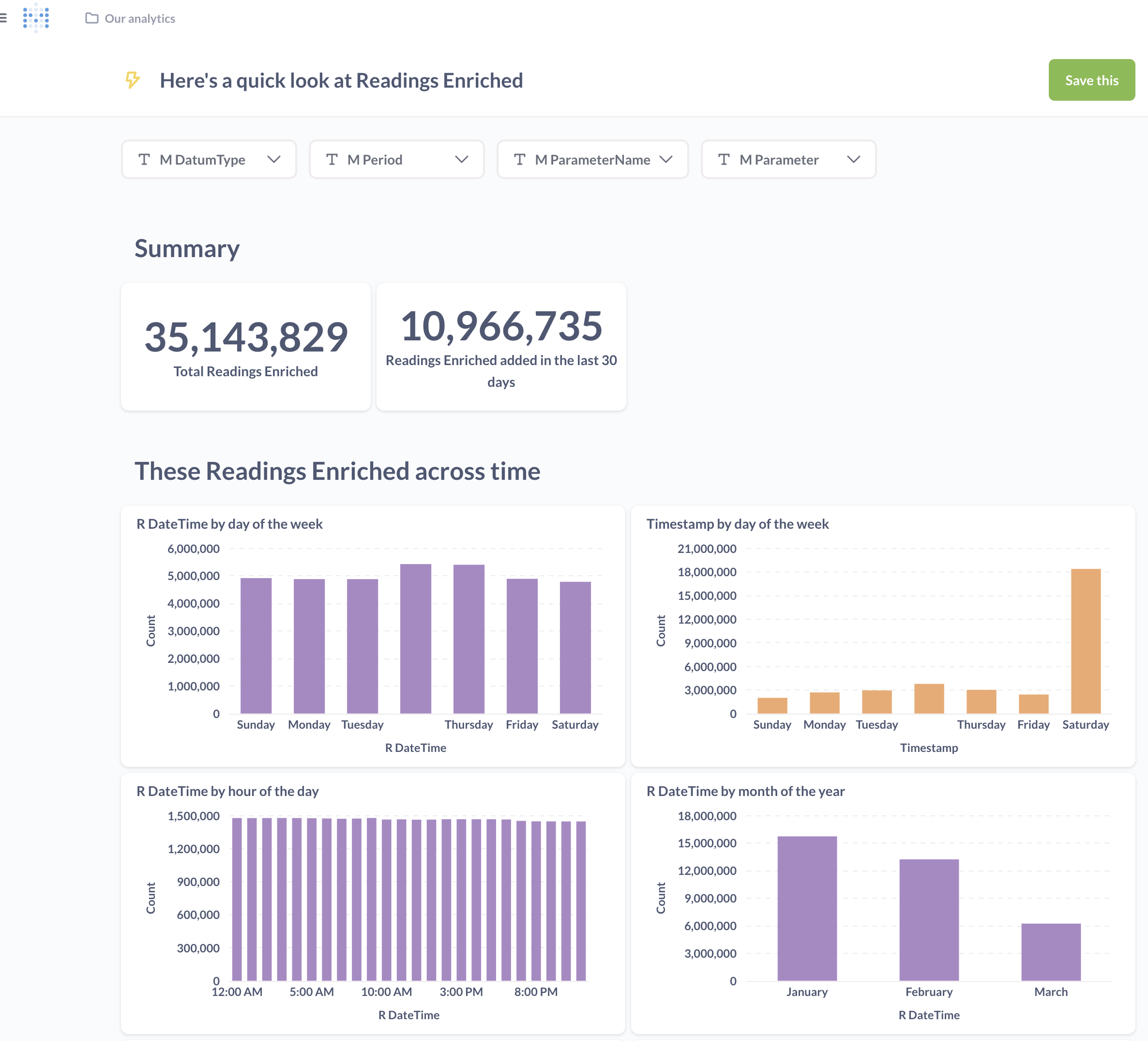
Once you’ve done that Metabase automagically (I’m surprised it doesn’t say "AI" when it does it) offers a summary of the data in the table:
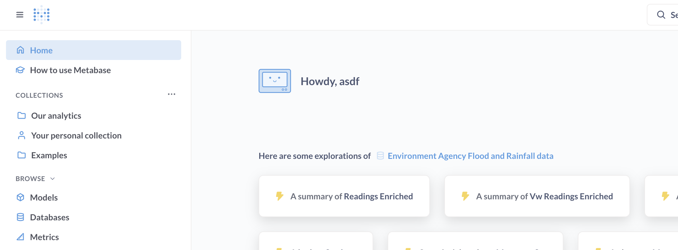
It’s not a bad starter for ten; the count of rows is useful from a data-completeness point of view.
We’d need to do some work to define the value metric and perhaps some geographic hierarchies—but there’s definitely lots of potential.
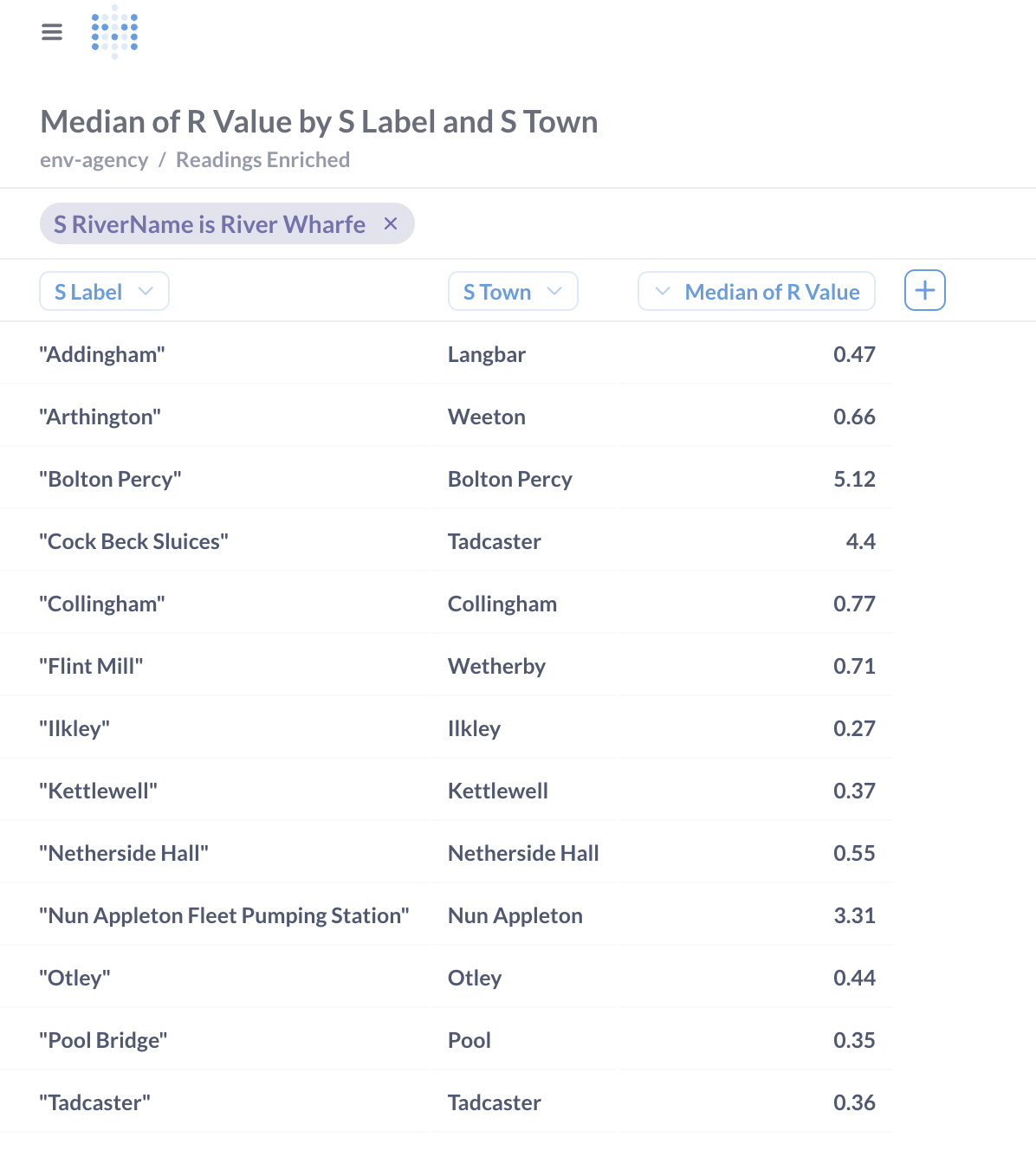
You can also poke around in the data itself with a tabular slice & dice approach:
Rill 🔗
I used Rill previously and liked it.
Getting it up and running is easy:
# Install…
curl https://rill.sh | sh
# …and go!
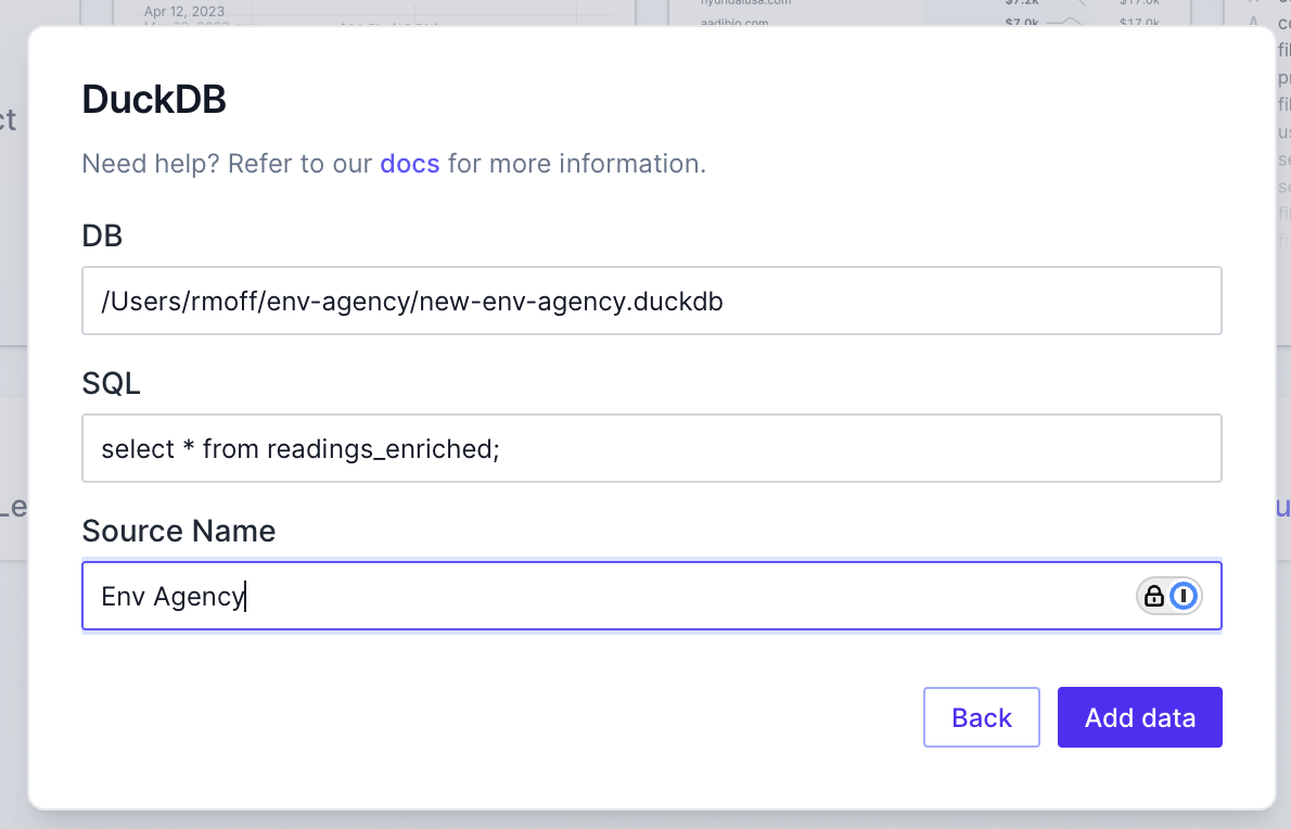
rill start rill-env-agencyRill supports DuckDB out of the box, so adding our data source is easy:
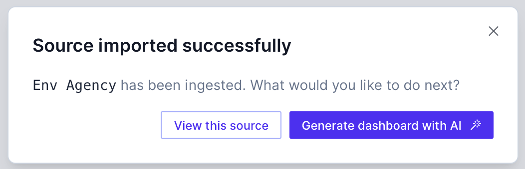
Who can resist a bit of AI magic?
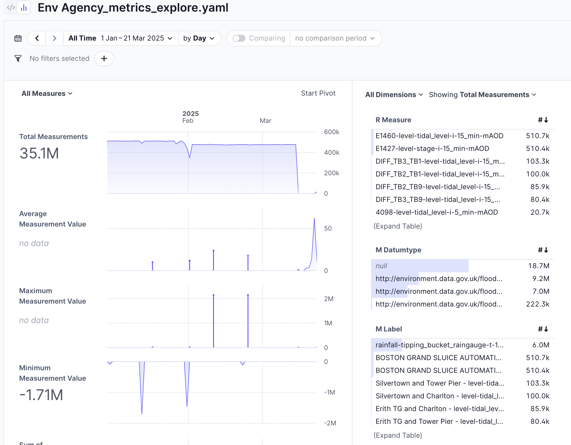
As with Metabase, it’s a pretty good starting point for customising into what you want to analyse.
With a bit of playing around you can create a nice comparison between January and February’s readings for stations on a given river:
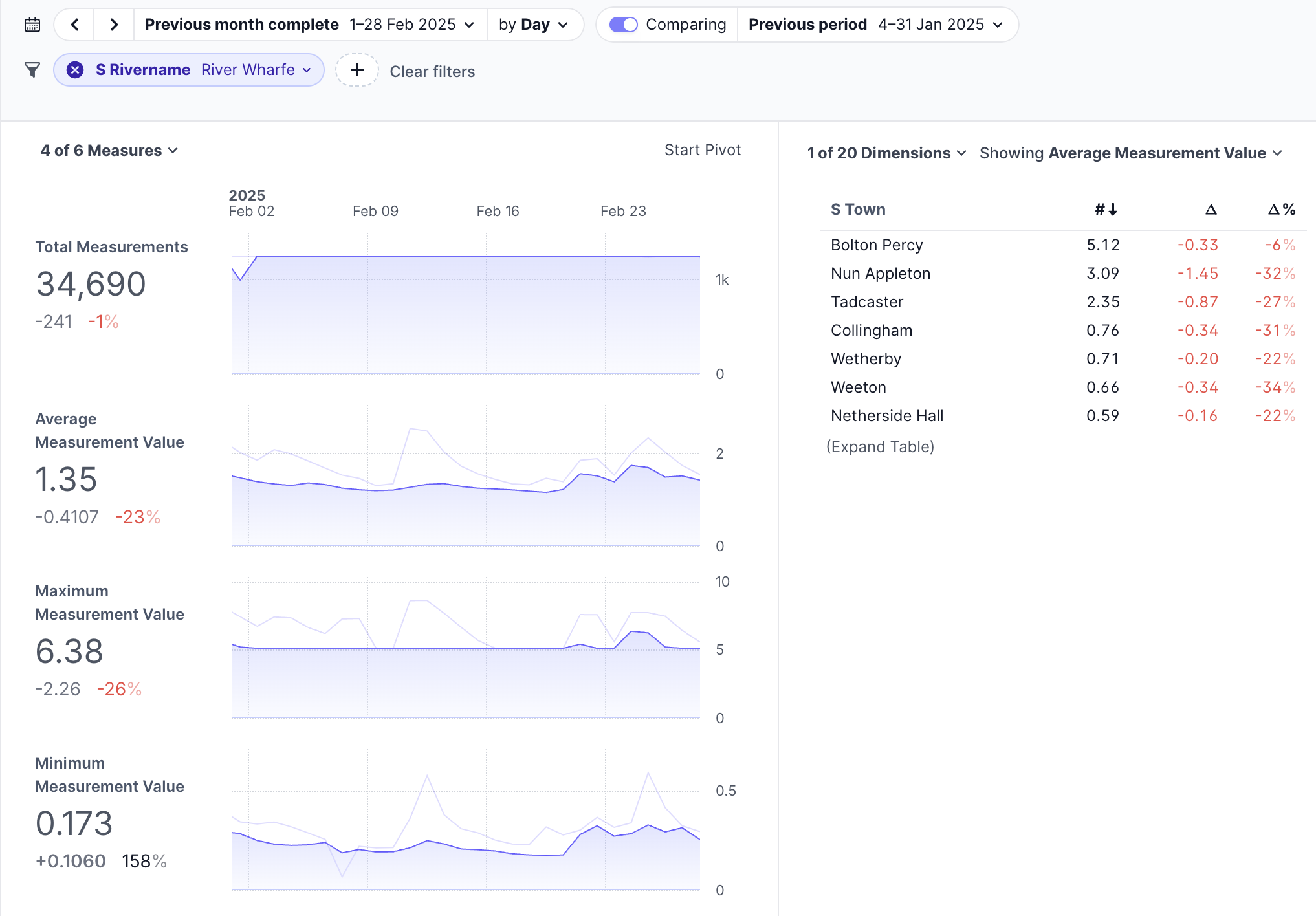
I couldn’t figure out how to plot a time series of values for a series of data, but as my children would say to me, that’s probably a skill issue on my part…
Superset 🔗
This is a bit heavier to install than Metabase, and definitely more so than Rill. After an aborted attempt to install it locally I went the Docker route even though it meant a bit of fiddling to get the DuckDB dependency installed.
Follow the steps in the Quickstart to clone the repo, and then modify the command for the superset service to install the DuckDB dependencies before launching Superset itself:
command: ["sh", "-c", "pip install duckdb duckdb-engine && /app/docker/docker-bootstrap.sh app-gunicorn"]Now bring up Superset:
docker compose -f docker-compose-image-tag.yml upYou’ll find Superset at http://localhost:8088—note that it does take a few minutes to boot up, so don’t be impatient if it doesn’t seem to be working straight away.
After quite a lot of fiddling around to get this far, I realised that my DuckDB file is on my host machine, not in the Docker container. I couldn’t just mount it as a volume as there are already volumes mounted using a syntax I wasn’t familiar with how to add to:
    volumes:
      *superset-volumes
Instead I just did a bit of a hack and copied the file onto the container:
docker compose cp ~/env-agency/env-agency.duckdb superset:/tmp/Finally, within Superset, I could add the database (Settings → Manage Databases).
Somewhat confusingly, if you select "DuckDB" as the type, you’re asked for "DuckDB Credentials" and a Motherduck access token; click the small Connect this database with a SQLAlchemy URI string instead link (or just select "Other" database type in the first place).
Specify the local path to your DuckDB file, for example:
duckdb:////tmp/env-agency.duckdb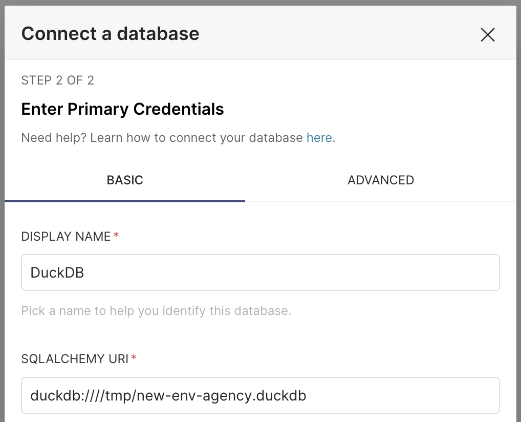
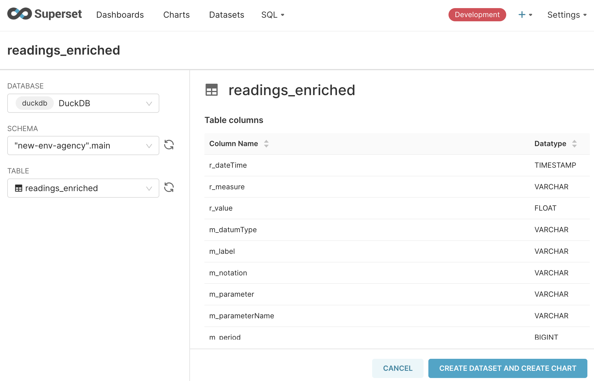
Next, create a Dataset—select the database you just defined, and the readings_enriched table:
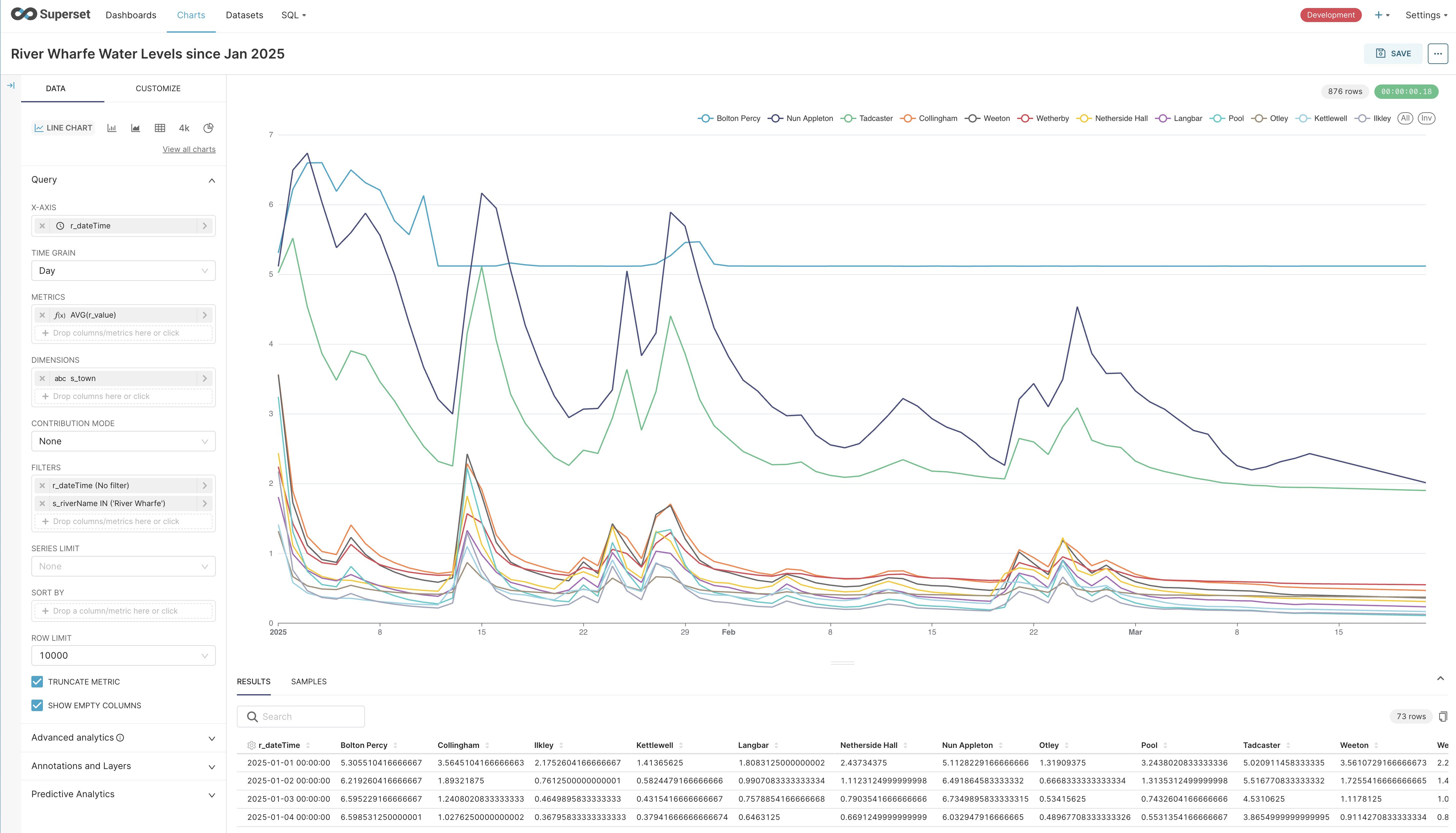
After all that, fortunately, Superset has a rich set of functionality particularly when it comes to charting. I did hit frequent time-outs when experimenting, but managed to create a nice time-series chart fairly easily:
Wrapping up 🔗
We’ve built cobbled together a pipeline that extracts data from a set of REST APIs, applies some light cleansing and transformation, and loads it into a DuckDB table from where it can be queried and analysed.
With cron we’ve automated the refresh of this data every fifteen minutes.
The total bill of materials is approximately:
-
1 x DuckDB
-
14 SQL statements (16 if you include historical backfill)
-
1 ropey cron job
Would this pass muster in a real deployment? You tell me :)
My guess is that I’d not want to be on the hook to support it, but it’d do the job until it didn’t. That is, as a prototype with sound modelling to expand on later it’s probably good enough.
But I’d love to hear from folk who are building this stuff for real day in, day out. What did I overlook here? Is doing it in DuckDB daft? Let me know on Bluesky or LinkedIn.
| You can find the full set of SQL files to run this here. |