
The UK Environment Agency publishes a feed of data relating to rainfall and river levels. As a prelude to building a streaming pipeline with this data, I wanted to understand the model of it first.
The API docs are pretty good, and from them I derived this model:

To poke around the data and make sure I understood how the different entities related, and what to expect from each API endpoint, I used DuckDB.
Load the data 🔗
The beauty of DuckDB is it is so simple, yet powerful. It generally behaves in a “oh cool, it just works” way. The data is published as JSON from a REST endpoint. To load it into DuckDB was just a case of using the read_json function:
CREATE TABLE readings_stg AS
    SELECT *
    FROM read_json('https://environment.data.gov.uk/flood-monitoring/data/readings');

CREATE TABLE measures_stg AS
    SELECT *
    FROM read_json('https://environment.data.gov.uk/flood-monitoring/id/measures');

CREATE TABLE stations_stg AS
    SELECT *
    FROM read_json('https://environment.data.gov.uk/flood-monitoring/id/stations');

CREATE TABLE floods_stg AS
    SELECT *
    FROM read_json('https://environment.data.gov.uk/flood-monitoring/id/floods');

CREATE TABLE floodAreas_stg AS
    SELECT *
    FROM read_json('https://environment.data.gov.uk/flood-monitoring/id/floodAreas');
🟡◗ show tables;
┌────────────────┐
│      name      │
│    varchar     │
├────────────────┤
│ floodAreas_stg │
│ floods_stg     │
│ measures_stg   │
│ readings_stg   │
│ stations_stg   │
└────────────────┘
The API returns three fields: @context, meta, and items. The latter is an array holding the actual payload. The meta field, as its name suggests, holds metadata.
🟡◗ describe readings_stg;
┌─────────────┬──────────────────────────────────────────────────────────────────────────────────────────────────────────────────────────────┬─────────┬─────────┬─────────┬─────────┐
│ column_name │                                                         column_type                                                          │  null   │   key   │ default │  extra  │
│   varchar   │                                                           varchar                                                            │ varchar │ varchar │ varchar │ varchar │
├─────────────┼──────────────────────────────────────────────────────────────────────────────────────────────────────────────────────────────┼─────────┼─────────┼─────────┼─────────┤
│ @context    │ VARCHAR                                                                                                                      │ YES     │ NULL    │ NULL    │ NULL    │
│ meta        │ STRUCT(publisher VARCHAR, licence VARCHAR, documentation VARCHAR, "version" VARCHAR, "comment" VARCHAR, hasFormat VARCHAR[]) │ YES     │ NULL    │ NULL    │ NULL    │
│ items       │ STRUCT("@id" VARCHAR, dateTime TIMESTAMP, measure VARCHAR, "value" DOUBLE)[]                                                 │ YES     │ NULL    │ NULL    │ NULL    │
└─────────────┴──────────────────────────────────────────────────────────────────────────────────────────────────────────────────────────────┴─────────┴─────────┴─────────┴─────────┘
Run Time (s): real 0.003 user 0.000728 sys 0.000293

🟡◗ select * from readings_stg;
┌──────────────────────┬──────────────────────┬───────────────────────────────────────────────────────────────────────────────────────────────────────────────────────────────────────────────────────────────────────────────────────────────────────────────────────────────────────────────────────────────────────────────┐
│       @context       │         meta         │                                                                                                                                     items                                                                                                                                     │
│       varchar        │ struct(publisher v…  │                                                                                                 struct("@id" varchar, datetime timestamp, measure varchar, "value" double)[]                                                                                                  │
├──────────────────────┼──────────────────────┼───────────────────────────────────────────────────────────────────────────────────────────────────────────────────────────────────────────────────────────────────────────────────────────────────────────────────────────────────────────────────────────────────────────────┤
│ http://environment…  │ {'publisher': Envi…  │ [{'@id': http://environment.data.gov.uk/flood-monitoring/data/readings/531166-level-downstage-i-15_min-mAOD/2025-02-28T00-00-00Z, 'dateTime': 2025-02-28 00:00:00, 'measure': http://environment.data.gov.uk/flood-monitoring/id/measures/531166-level-downstage-i-15_min-m…  │
└──────────────────────┴──────────────────────┴──────────────────────────────────────────────────────────────────────────────────────────────────────────────────────────────────────────────────────────────────────────────────────────────────────────────────────────────────────────────────────────────────────────────┘
Explore the JSON array 🔗
To get at the data I exploded out the JSON items array.
CREATE TABLE stations AS
	SELECT u.* FROM
		(SELECT UNNEST(items) AS u FROM stations_stg);
🟡◗ DESCRIBE stations;
┌──────────────────┬───────────────────────────────────────────────────────────────────────────────────────────────────────────────────────┬─────────┬─────────┬─────────┬─────────┐
│   column_name    │                                                      column_type                                                      │  null   │   key   │ default │  extra  │
│     varchar      │                                                        varchar                                                        │ varchar │ varchar │ varchar │ varchar │
├──────────────────┼───────────────────────────────────────────────────────────────────────────────────────────────────────────────────────┼─────────┼─────────┼─────────┼─────────┤
│ @id              │ VARCHAR                                                                                                               │ YES     │         │         │         │
│ RLOIid           │ JSON                                                                                                                  │ YES     │         │         │         │
│ catchmentName    │ JSON                                                                                                                  │ YES     │         │         │         │
│ dateOpened       │ DATE                                                                                                                  │ YES     │         │         │         │
│ easting          │ JSON                                                                                                                  │ YES     │         │         │         │
│ label            │ JSON                                                                                                                  │ YES     │         │         │         │
│ lat              │ JSON                                                                                                                  │ YES     │         │         │         │
│ long             │ JSON                                                                                                                  │ YES     │         │         │         │
│ measures         │ STRUCT("@id" VARCHAR, parameter VARCHAR, parameterName VARCHAR, period BIGINT, qualifier VARCHAR, unitName VARCHAR)[] │ YES     │         │         │         │
│ northing         │ JSON                                                                                                                  │ YES     │         │         │         │
│ notation         │ VARCHAR                                                                                                               │ YES     │         │         │         │
│ riverName        │ VARCHAR                                                                                                               │ YES     │         │         │         │
│ stageScale       │ VARCHAR                                                                                                               │ YES     │         │         │         │
│ stationReference │ VARCHAR                                                                                                               │ YES     │         │         │         │
│ status           │ JSON                                                                                                                  │ YES     │         │         │         │
│ town             │ VARCHAR                                                                                                               │ YES     │         │         │         │
│ wiskiID          │ VARCHAR                                                                                                               │ YES     │         │         │         │
│ datumOffset      │ DOUBLE                                                                                                                │ YES     │         │         │         │
│ gridReference    │ VARCHAR                                                                                                               │ YES     │         │         │         │
│ downstageScale   │ VARCHAR                                                                                                               │ YES     │         │         │         │
├──────────────────┴───────────────────────────────────────────────────────────────────────────────────────────────────────────────────────┴─────────┴─────────┴─────────┴─────────┤
│ 20 rows                                                                                                                                                                6 columns │
└──────────────────────────────────────────────────────────────────────────────────────────────────────────────────────────────────────────────────────────────────────────────────┘
We can now query it as a ‘regular’ table:
🟡◗ select * from stations limit 1;
┌──────────────────────┬────────┬───────────────┬────────────┬─────────┬───────────────────┬───────────┬───────────┬──────────────────────┬──────────┬──────────┬──────────────┬──────────────────────┬──────────────────┬───────────────────────┬───────────────────┬─────────┬─────────────┬───────────────┬────────────────┐
│         @id          │ RLOIid │ catchmentName │ dateOpened │ easting │       label       │    lat    │   long    │       measures       │ northing │ notation │  riverName   │      stageScale      │ stationReference │        status         │       town        │ wiskiID │ datumOffset │ gridReference │ downstageScale │
│       varchar        │  json  │     json      │    date    │  json   │       json        │   json    │   json    │ struct("@id" varch…  │   json   │ varchar  │   varchar    │       varchar        │     varchar      │         json          │      varchar      │ varchar │   double    │    varchar    │    varchar     │
├──────────────────────┼────────┼───────────────┼────────────┼─────────┼───────────────────┼───────────┼───────────┼──────────────────────┼──────────┼──────────┼──────────────┼──────────────────────┼──────────────────┼───────────────────────┼───────────────────┼─────────┼─────────────┼───────────────┼────────────────┤
│ http://environment…  │ "7041" │ "Cotswolds"   │ 1994-01-01 │ 417990  │ "Bourton Dickler" │ 51.874767 │ -1.740083 │ [{'@id': http://en…  │ 219610   │ 1029TH   │ River Dikler │ http://environment…  │ 1029TH           │ "http://environment…  │ Little Rissington │ 1029TH  │             │               │                │
└──────────────────────┴────────┴───────────────┴────────────┴─────────┴───────────────────┴───────────┴───────────┴──────────────────────┴──────────┴──────────┴──────────────┴──────────────────────┴──────────────────┴───────────────────────┴───────────────────┴─────────┴─────────────┴───────────────┴────────────────┘
Run Time (s): real 0.006 user 0.002751 sys 0.001281
I ran the same UNNEST for all the tables:
CREATE TABLE stations AS
    SELECT u.*
    FROM (SELECT UNNEST(items) AS u FROM stations_stg);

CREATE TABLE measures AS
    SELECT u.*
    FROM (SELECT UNNEST(items) AS u FROM measures_stg);

CREATE TABLE readings AS
    SELECT u.*
    FROM (SELECT UNNEST(items) AS u FROM readings_stg);

CREATE TABLE floods AS
    SELECT u.*
    FROM (SELECT UNNEST(items) AS u FROM floods_stg);

CREATE TABLE floodAreas AS
    SELECT u.*
    FROM (SELECT UNNEST(items) AS u FROM floodAreas_stg);
Which then gave me ten tables in total:
🟡◗ SHOW TABLES;
┌────────────────┐
│      name      │
│    varchar     │
├────────────────┤
│ floodAreas     │
│ floodAreas_stg │
│ floods         │
│ floods_stg     │
│ measures       │
│ measures_stg   │
│ readings       │
│ readings_stg   │
│ stations       │
│ stations_stg   │
├────────────────┤
│    10 rows     │
└────────────────┘
Join the data 🔗
There are, I think, two main sets of fact data—readings and floods. Looking at the former, I joined the three main tables using the data model I derived from the API reference :
SELECT
      "r_\0": COLUMNS(r.*),
      "m_\0": COLUMNS(m.*),
      "s_\0": COLUMNS(s.*)
       FROM
      readings r
      INNER JOIN m:measures ON r.measure = m."@id"
      INNER JOIN s:stations ON m.station = s."@id"
    LIMIT 1;
The COLUMNS expression is detailed here and the prefix aliases here.
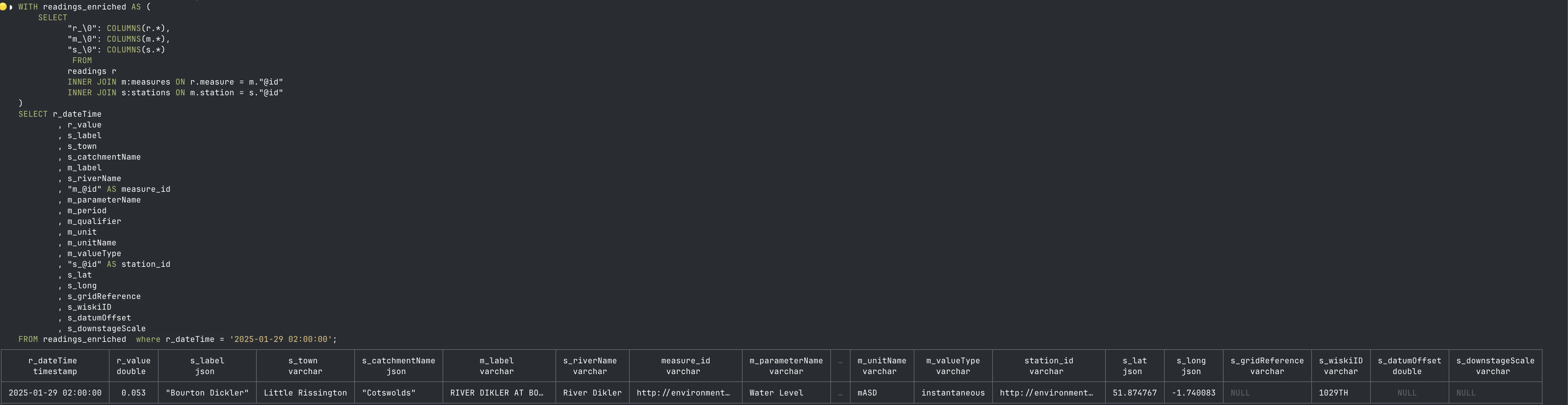
This seemed to work, so next up I wanted to examine the actual data. Looking down each table I picked out the fields that looked relevant to being able to answer the question “what is this reading, and where is it from”?
WITH readings_enriched AS (
	SELECT
	      "r_\0": COLUMNS(r.*),
	      "m_\0": COLUMNS(m.*),
	      "s_\0": COLUMNS(s.*)
	       FROM
	      readings r
	      INNER JOIN m:measures ON r.measure = m."@id"
	      INNER JOIN s:stations ON m.station = s."@id"
)
SELECT r_dateTime
		, r_value
		, s_label
		, s_town
		, s_catchmentName
		, m_label
		, s_riverName
		, "m_@id" AS measure_id
		, m_parameterName
		, m_period
		, m_qualifier
		, m_unit
		, m_unitName
		, m_valueType
		, "s_@id" AS station_id
		, s_lat
		, s_long
		, s_gridReference
		, s_wiskiID
		, s_datumOffset
		, s_downstageScale
FROM readings_enriched;
If you get into the data in depth you’ll notice some repetition amongst it—for example, measures also includes latestReading. Part of my exploration was to understand the grain of the data in each table and where any duplication might occur in results.
With a monitor that is only so wide, and a slightly vague requirement for looking at the data (which thus ruled out crafting some SQL with GROUP BY etc to break it down), I reached for some graphical exploration.
Visualising the data with Rill 🔗
After an unsuccessful foray with datasette (cool tool, but based on SQLite and even with datasette-parquet not very happy with running my queries) I tried out Rill, which had been recommended to me by Simon Späti. The installation is ridiculously simple:
curl rill.sh | sh && rill start
Then create a source definition for each of the tables:
# Source YAML
# Reference documentation: https://docs.rilldata.com/reference/project-files/sources

type: source

connector: "duckdb"
db: "/Users/rmoff/work/environment.data.gov.uk/env-agency.duckdb"
sql: "select * from measures;"
As soon as you create the definition it pulls in the data and gives you a nice summary of it:
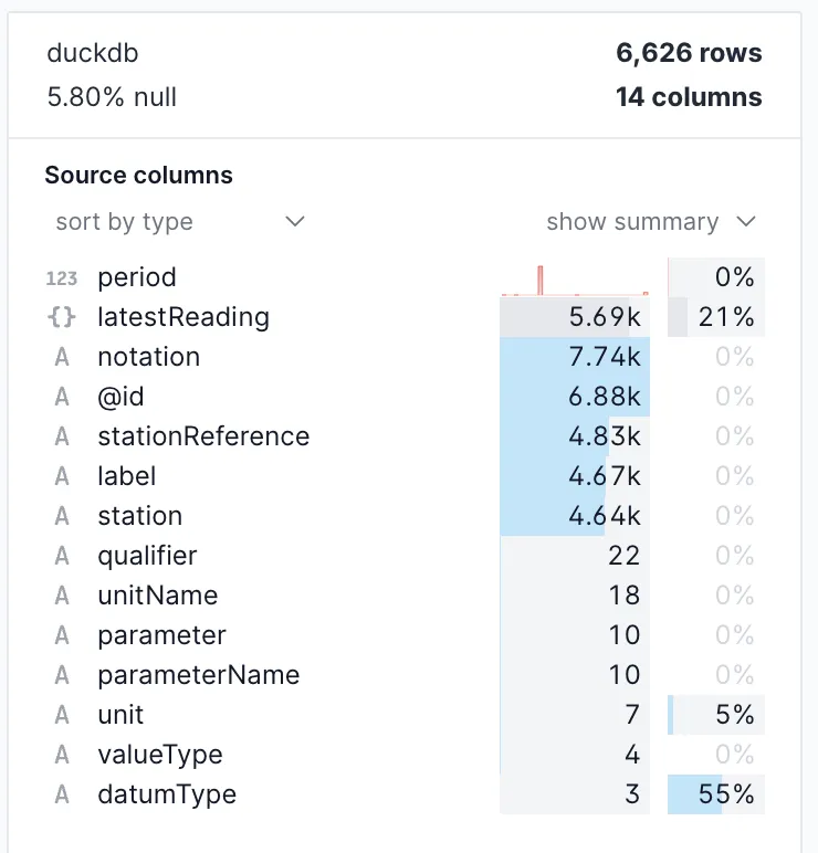
Clicking on a field gives you a breakdown of its values:

In this example, the parameter field has 10 unique values (per the first screenshot), and within it nearly four in five are for level, followed by rainfall (second screenshot).
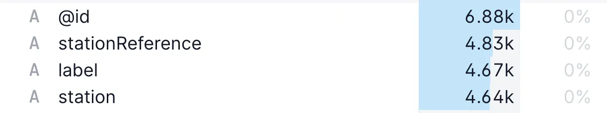
Within the measures data we can also discern information about the granularity. Whilst there are 6.8k @id (the unique key, I think?) values, there are only 4.6k unique stations.
 Within this, there are usually 6 measures per station, although sometimes 8 or 12:
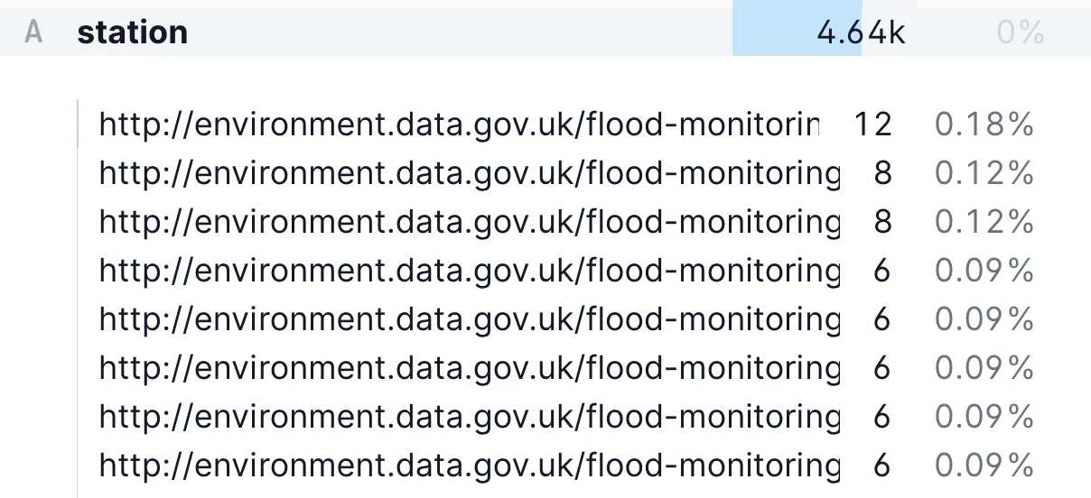
The value repeats because the unique station ID is on the end of the URL—a quick SPLIT function demonstrates that:
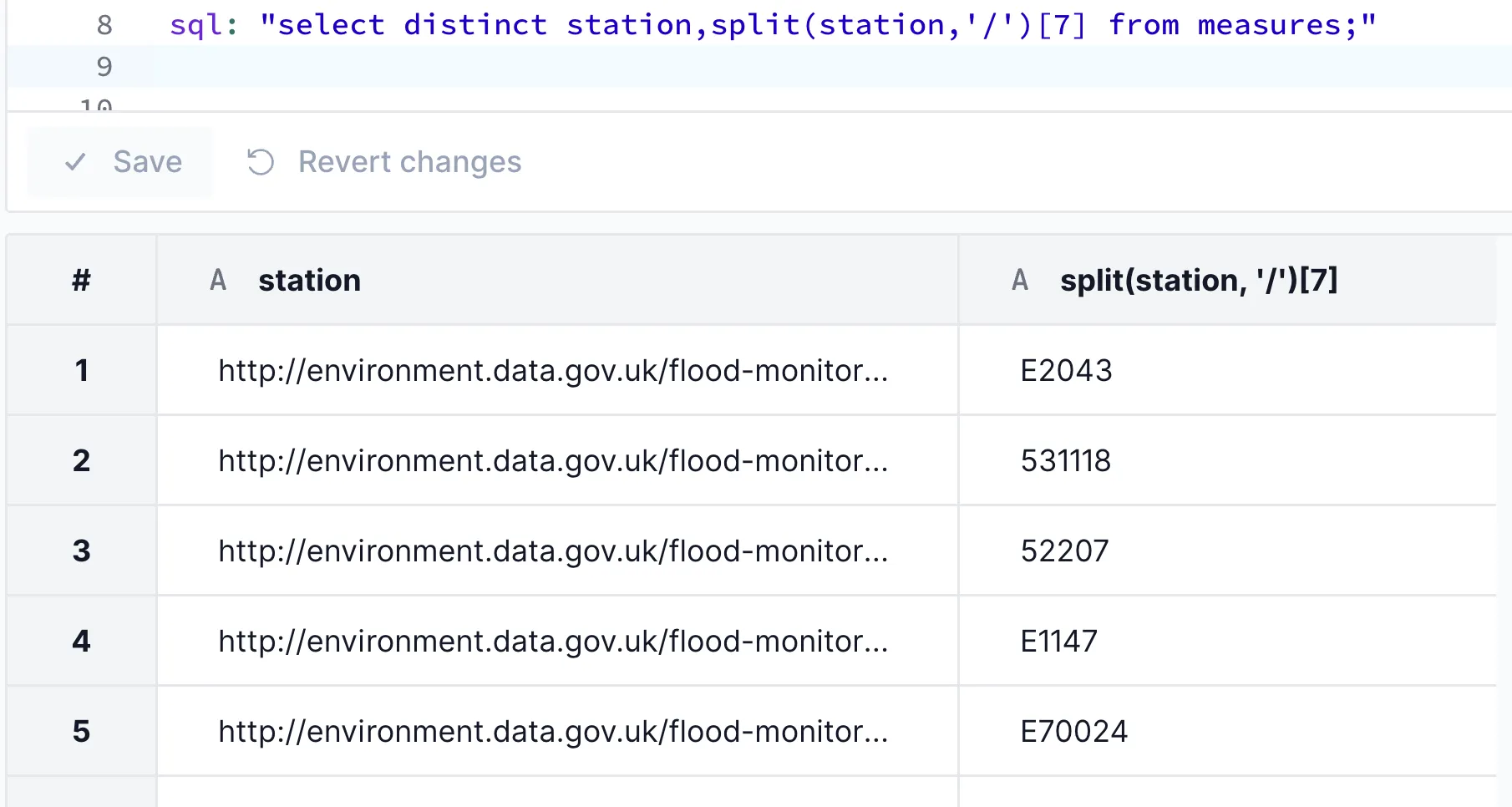
That’s measures broadly understood - each measure is unique, and relates to a station. Each station can have multiple measures. What about readings?
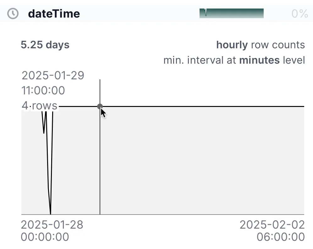
Rill makes life so easy here. There’s just over five days’ worth of data, and there are usually four rows per hour:
However, we might have something of interest here:
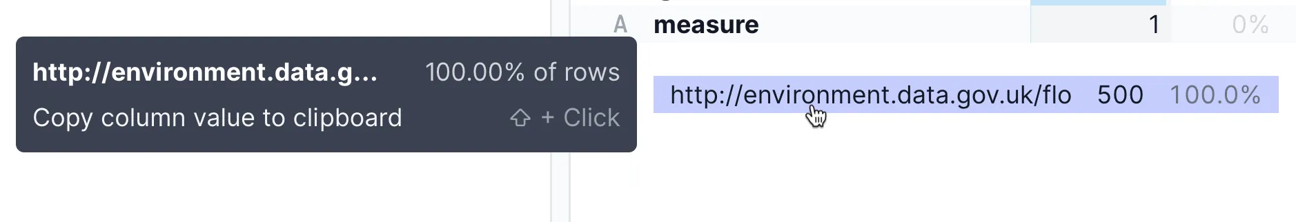
Within all the readings data, there’s only one measure:
http://environment.data.gov.uk/flood-monitoring/id/measures/1029TH-level-downstage-i-15_min-mASD
As we’ve seen above, a measure is unique to a station and type of measurement at that station.
From here, in Rill I created a model - no idea what one was, but there was a button to click. It seems to let you write SQL against the sources defined:
SELECT * FROM
	      readings r
	      INNER JOIN measures m ON r.measure = m."@id"
	      INNER JOIN stations s ON m.station = s."@id"
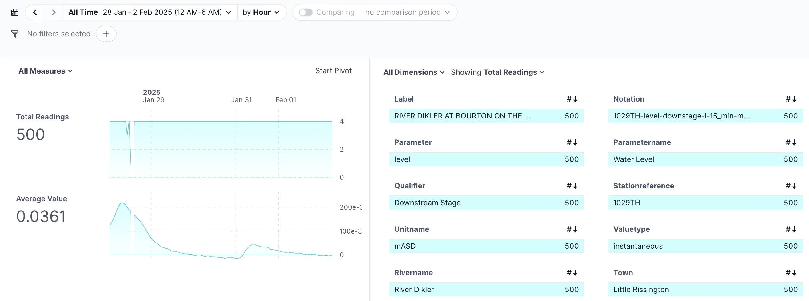
After a bit of fiddling to remove duplicate fields I had a button to click next to the model to automagically (“with AI” oooooooh!) generate a dashboard—it’d have been rude not to try it…

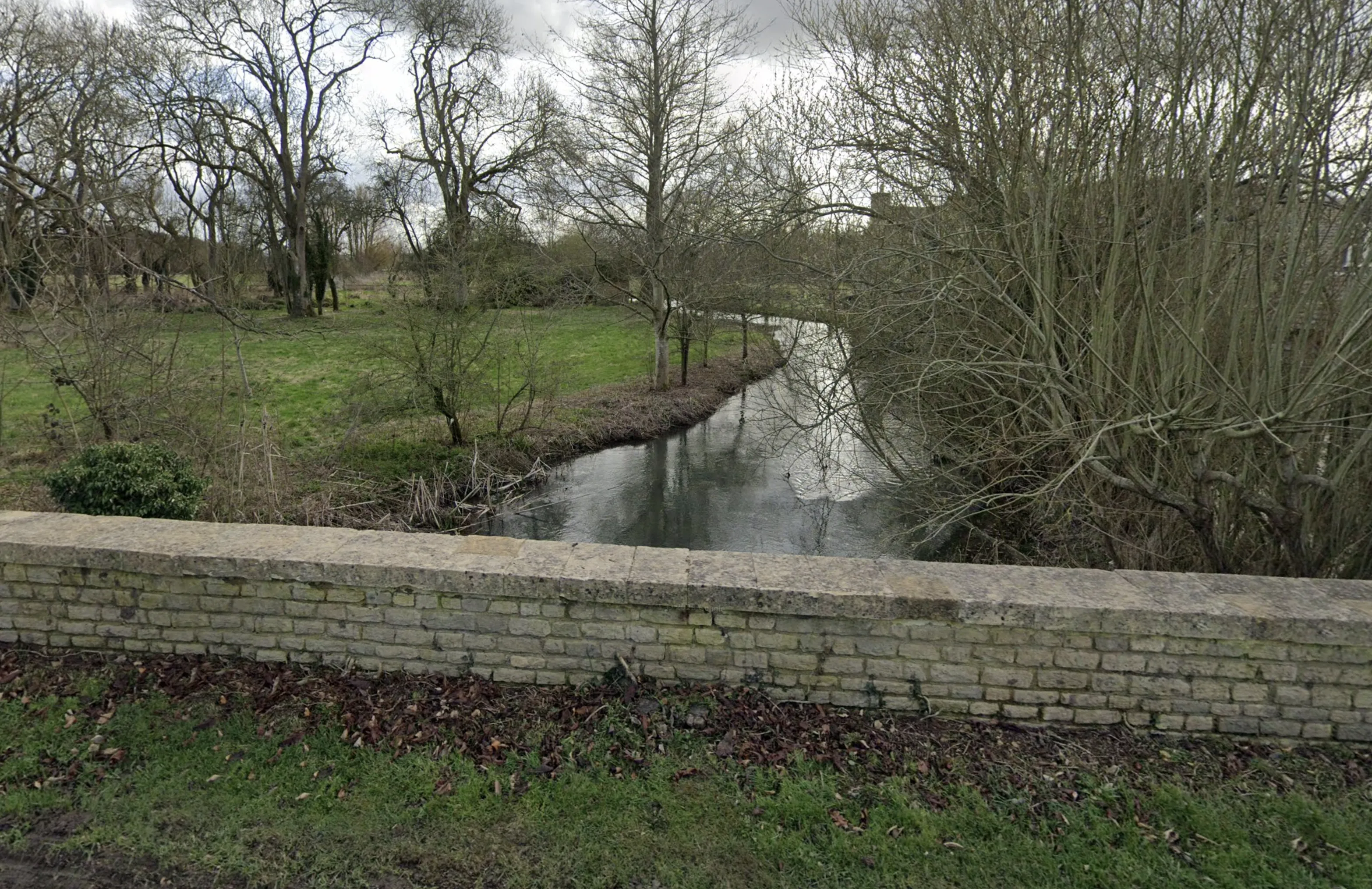
And thus, a nice illustration of the hourly water level on the River Dikler in Little Rissington
Where are the rest of the readings? 🔗
As we saw above, there are 500 readings, all for measure level-downstage-i-15_min-mASD at station 1029TH (on the River Dikler, above).
But what about all the others?
Per the API docs, there is a default limit of 500 records from the readings endpoint. Let’s look more closely at the URL I used to load the data into DuckDB originally:
CREATE TABLE readings_stg AS
    SELECT *
    FROM read_json('https://environment.data.gov.uk/flood-monitoring/data/readings');
We can see that it is missing the ?latest parameter, meaning that it’ll pull everything—up to a limit of 500 records. Which is precisely what we’ve seen above—but it’s easy to miss when in the depths of a new dataset and dozens of columns. A graphical view of the data helps a lot to whittle these things down.
Let’s replace the data into the readings_stg table and use the ?today parameter which should hopefully pull multiple time samples across all stations and measurements this time:
CREATE OR REPLACE TABLE readings_stg AS
    SELECT *
    FROM read_json('https://environment.data.gov.uk/flood-monitoring/data/readings?today');
Well, we’re definitely getting more data!
Run Time (s): real 11.356 user 0.236345 sys 0.286720
Invalid Input Error:
"maximum_object_size" of 16777216 bytes exceeded while reading file "https://environment.data.gov.uk/flood-monitoring/data/readings?today" (>33554428 bytes).
 Try increasing "maximum_object_size".
The default for maximum_object_size is 16777216 bytes, or 16MB. Let’s pump those rookie numbers up:
🟡◗ CREATE OR REPLACE TABLE readings_stg AS
        SELECT *
        FROM READ_JSON('https://environment.data.gov.uk/flood-monitoring/data/readings?today',
                        maximum_object_size=67108864);
Run Time (s): real 3.758 user 0.656197 sys 0.410768
Now rebuild the readings table (I guess we could build this into one SQL statement, but then we lose the visibility and ability to debug each stage of transformation):
CREATE OR REPLACE TABLE readings AS
    SELECT u.*
    FROM (SELECT UNNEST(items) AS u FROM readings_stg);
We’ve got over 170k readings:
🟡◗ SELECT COUNT(*) FROM readings;
┌──────────────┐
│ count_star() │
│    int64     │
├──────────────┤
│    170841    │
└──────────────┘
Let’s head back to Rill (after closing my DuckDB CLI session, since two sources can’t work with the DB by default) to see what the updated readings data looks like:
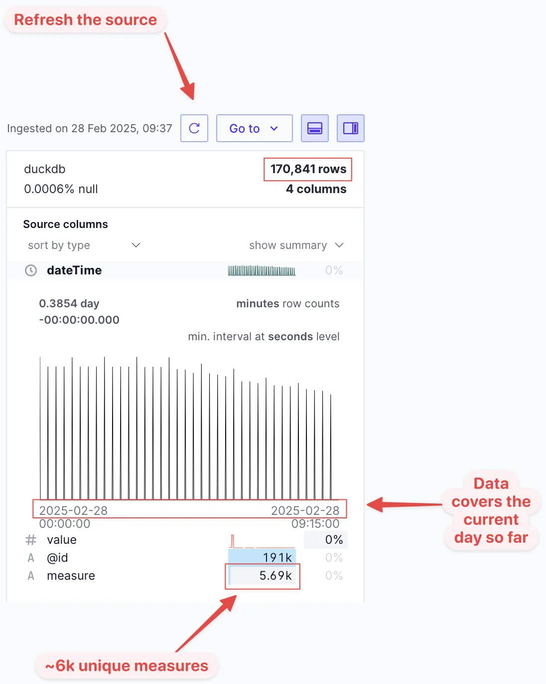 This looks much more complete. There’s data from the beginning of today up until just now when I ran the query. If I were running this as a continual ingest I’d use the
 ?latest endpoint to not pull in the data from earlier in the day.
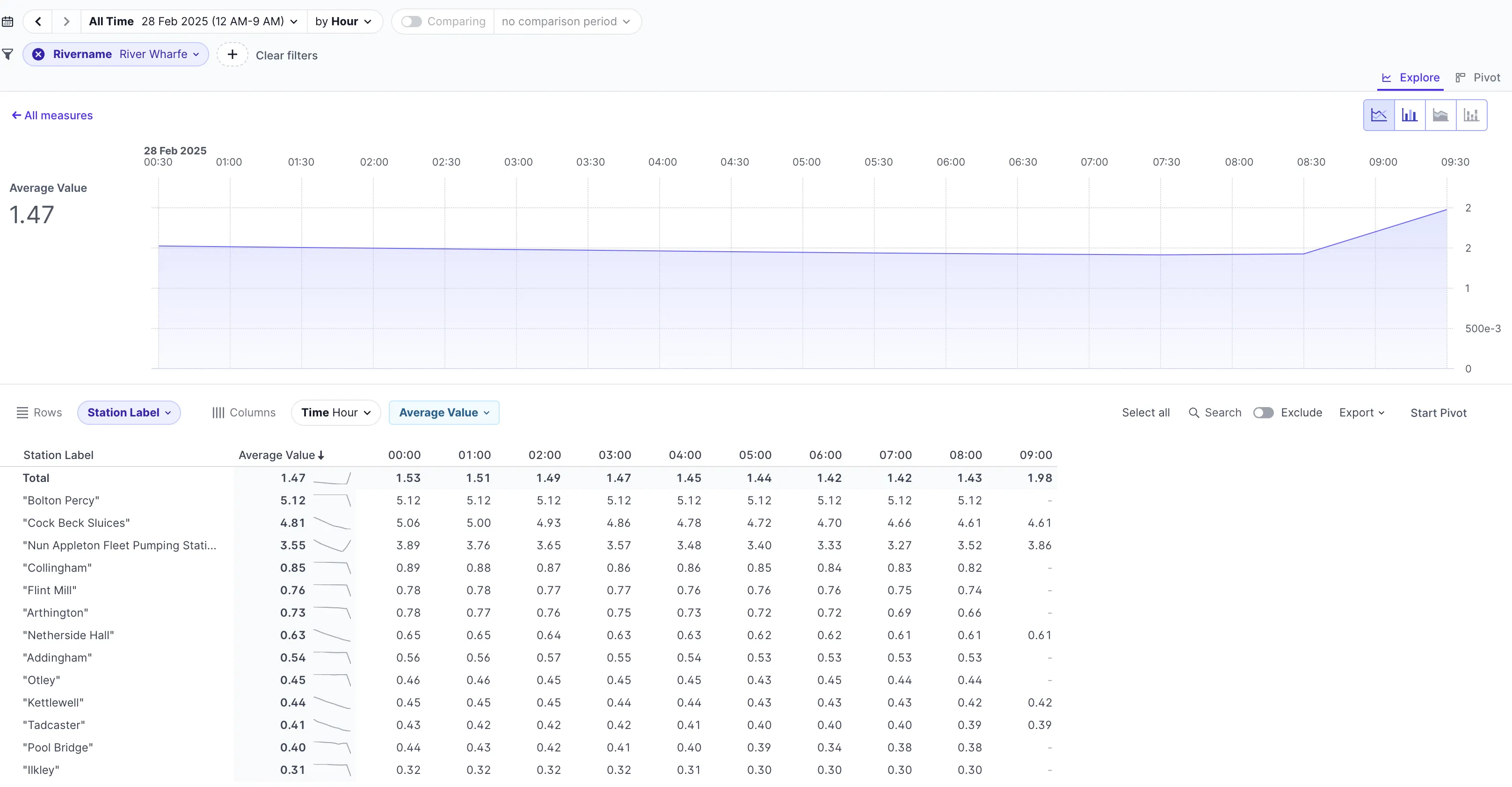
On the dashboard we now have all the different stations, and can start to really slice and dice the data. Here it is filtered by the Rivername, showing just stations on the River Wharfe:
Summary 🔗
So, that was fun :) DuckDB is just the best for rapid ingest and prototyping with data, and Rill proved itself out to be not only pretty intuitive to use and fast (unsurprising, since it’s built on DuckDB itself)— but also exactly what I was looking for in a tool to quickly visualise data to understand it better. If you’re interested in what other tools people suggested for this task check out this BlueSky thread.
Data attribution: This uses Environment Agency flood and river level data from the real-time data API (Beta), provided under the Open Government Licence.