Data Wrangling with Flink SQL

The UK Government publishes a lot of its data as open feeds. One that I keep coming back to is the Environment Agency’s flood-monitoring API that gives access to an estate of sensors that provide information about data such as river levels and rainfall.

The data is well-structured and provided across three primary API endpoints. In this blog article I’m going to show you how I use Flink SQL to explore and wrangle these into the kind of form from which I am then going to build a streaming pipeline using them.

I initially used DuckDB and Rill Data to explore the structure of the data and verify the relationships and keys.

4a663670f62f9acd7d15158b64bfa417.excalidraw

Now to work with it in Apache Flink :)

The data is loaded into three Apache Kafka topics, each corresponding to the respective API.

The first step was to unnest the source data, each of which uses an items array to nest the actual payload. I wrote about how to do this here. It’s done with CROSS JOIN UNNEST in Flink SQL:

CREATE TABLE readings AS
	SELECT meta.publisher, meta.version, i.dateTime, i.measure, i.`value`
      FROM `flood-monitoring-readings` r
	  CROSS JOIN UNNEST(r.items) AS i;

CREATE TABLE `measures` AS
	SELECT meta.publisher, meta.version, i.*
     FROM `flood-monitoring-measures` m
	  CROSS JOIN UNNEST(m.items) AS i;

CREATE TABLE stations AS
	SELECT meta.publisher, meta.version, i.*
     FROM `flood-monitoring-stations` s
	  CROSS JOIN UNNEST(s.items) AS i;

This results in three new Flink tables, backed by Kafka topics:

readings

{
  "publisher": "Environment Agency",
  "version": "0.9",
  "dateTime": 1740380400000,
  "measure": "http://environment.data.gov.uk/flood-monitoring/id/measures/SU89_82-level-groundwater-i-1_h-mAOD",
  "value": 50.211
}

measures

{
  "publisher": "Environment Agency",
  "version": "0.9",
  "label": "Leeds FAS Calverley FSR Upstream Level - level-stage-i-15_min-mAOD",
  "parameterName": "Water Level",
  "unitName": "mAOD",
  "valueType": "instantaneous"
  […]

stations

{
  "publisher": "Environment Agency",
  "version": "0.9",
  "label": "Hurworth",
  "notation": "L3609A",
  "riverName": {
    "string": "River Tees"
  },
  "gridReference": {
    "string": "NZ3108210067"
  },
  "lat": {
    "string": "54.484987"
  },
  "long": {
    "string": "-1.521745"
  },
[…]

The Plan 🔗

Going back to my roots as a data engineer, there were several things I wanted to do with the data:

Not all the fields in items or meta arrays are directly useful, so I’d like to exclude them from the downstream pipeline. However, typing out the full list of columns except those you don’t want is not only time consuming, but hugely error prone. It also makes future schema evolution more difficult, because if you add (or remove) a column in the future, you need to make sure that all down-stream processes do the same, otherwise you will lose (or incorrectly try to query) the new column.

DuckDB supports a SELECT * EXCLUDE (except_this_column) syntax; unfortunately Flink SQL doesn’t. So, we can scratch that one off the list for now.
The meta field in each API response is useful, but doesn’t necessarily belong in the payload; it’s what Kafka headers are useful for. So can we do that with Flink SQL?
Whilst readings are facts/events, the stations and measures are dimensions/reference data. Each time we poll the API we get a full dump of the reference data. I want to work out how to logically model (primary/foreign keys) and physically store (compacted topics?) this in Flink and Kafka.
Finally, once we’ve done this, what does joining the three entities in Flink SQL look like?

Writing Kafka headers from Flink SQL 🔗

With each request is included a meta array of data. It’d be nominally useful to know, but included in the main payload makes it even wider that it is already.

"meta" : {
    "publisher": "Environment Agency",
    "version": "0.9",
    "licence" : "http://www.nationalarchives.gov.uk/doc/open-government-licence/version/3/" ,
    "documentation" : "http://environment.data.gov.uk/flood-monitoring/doc/reference" ,
    "version" : "0.9" ,
    "comment" : "Status: Beta service" ,
    […]

This is a perfect fit for record headers in Kafka.

To include them in a Flink table backed by a Kafka topic, use a headers metadata column.

First, I’ll create a new table into which to write the readings data, based on the existing one:

CREATE TABLE readings_with_header AS
	SELECT `dateTime`, `measure` , `value` FROM readings LIMIT 0;

Then add the headers column—note the METADATA keyword.

ALTER TABLE `readings_with_header`
	ADD headers MAP<STRING NOT NULL, STRING NOT NULL> METADATA;

So now the table looks like this:

DESCRIBE `readings_with_header`;

  Column Name      Data Type                               Nullable   Extras
--------------+------------------------------------------+----------+-----------
  dateTime      TIMESTAMP_LTZ(3)                           NOT NULL
  measure       STRING                                     NOT NULL
  value         DOUBLE                                     NOT NULL
  headers       MAP<VARCHAR(9) NOT NULL, STRING NOT NULL>  NULL      METADATA

To add data into it we’ll copy it across from the previous incarnation of the table. Note how the headers are specified as a key/value—the key is the column name, the value is the column value itself:

INSERT INTO `readings_with_header`
	SELECT `dateTime`, `measure`, `value`,
		MAP['publisher', publisher,
                    'version', version]      AS headers
	  FROM `readings`;

With the data in the table, let’s take a look at the underlying Kafka topic. I’m going to use one of my favourite tools: kcat.

$ kcat -C -t readings_with_header -c1 -s avro -f '\nKey (%K bytes): %k
  Value (%S bytes): %s
  Timestamp: %T
  Partition: %p
  Offset: %o
  Headers: %h\n'

Key (-1 bytes):
Value (72 bytes): {"dateTime": 1740562200000, "measure": "1023SE-rainfall-tipping_bucket_raingauge-t-15_min-mm", "value": 0.0}
Timestamp: 1741615690391
Partition: 2
Offset: 0
Headers: version=0.9,publisher=Environment Agency

I’m using a kcat config file (~/.config/kcat.conf) to hold details of my broker and credentials etc. Read more about it here.

Learn more about headers and other Kafka metadata available in Flink here and here.

Handling dimensions in Flink SQL 🔗

Setting the Kafka record key 🔗

As you can see in the output from kcat above, there are no keys currently set on the Kafka messages:

Key (-1 bytes):

Let’s create a new version of the measures table with a primary key (PK). This uses the PRIMARY KEY and DISTRIBUTED BY syntax. The primary key is set as id, which is an alias for the original @id column (changed to _40id at ingest). The column projection is restated here (instead of a SELECT *) to change the order of columns so that the PK is the first column in the table.

CREATE TABLE measure_with_pk
	(PRIMARY KEY (`id`) NOT ENFORCED)
	DISTRIBUTED BY HASH(`id`) INTO 6 BUCKETS
     AS SELECT  	`_40id` as `id`,
			datumType,
			label,
			notation,
			`parameter`,
			parameterName,
			`period`,
			qualifier,
			station,
			stationReference,
			unit,
			unitName,
			valueType
          FROM `measures`;

Now the key of a Kafka message from the topic underpinning the table looks like this:

$ kcat -C -t measure_with_pk -c1 \
       -s avro -f '\nKey (%K bytes): %k\nValue (%S bytes): %s'

Key (95 bytes): {"id": "http://environment.data.gov.uk/flood-monitoring/id/measures/50150-level-stage-i-15_min-m"}
Value (222 bytes): {"datumType": null, "label": "BRENDON - level-stage-i-15_min-m", "notation": "50150-level-stage-i-15_min-m", "parameter": "level", "parameterName": "Water Level", "period": {"int": 900}, "qualifier": "Stage", "station": "http://environment.data.gov.uk/flood-monitoring/id/stations/50150", "stationReference": "50150", "unit": {"string": "http://qudt.org/1.1/vocab/unit#Meter"}, "unitName": "m", "valueType": "instantaneous"}

Docs for primary keys and partitioning of Kafka topics with Flink tables here, here, and here.

Changing the Kafka topic under a Flink table to compacted 🔗

Kafka topic compaction is one of those wonderfully simple-yet-powerful concepts. Instead of an infinite append-only log, a compacted topic starts to feel more like regular RDBMS table. For each key (hence the importance of setting them correctly in the section above), Kafka will retain the latest value. To change the value for a key, you add another message to the topic with the same key. When the compaction process runs, it’ll remove earlier versions. You can also delete a key by sending a tombstone message, which is the key with a null for its value.

In short, a compacted topic is perfect for our reference data here. Whilst we could build the processing to handle changing values for our dimension data, we’re going to keep things very simple to start with. We’ll implement what is known as a Type 1 Slowly Changing Dimension (SCD). In essence, when we get a new (or unchanged) value for a dimension, we just replace the previous one.

Topic compaction is a Kafka topic configuration, so can be set as part of the connection properties in the CREATE TABLE statement:

CREATE TABLE measures_with_pk
	(PRIMARY KEY (`id`) NOT ENFORCED)
	DISTRIBUTED BY HASH(`id`) INTO 6 BUCKETS
	WITH ('kafka.cleanup-policy' = 'compact')
	AS SELECT  	`_40id` as `id`,
			datumType,
			label,
			notation,
			`parameter`,
			parameterName,
			`period`,
			qualifier,
			station,
			stationReference,
			unit,
			unitName,
			valueType
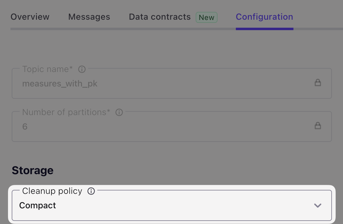
	FROM `measures`;

Over in the Confluent Cloud UI we can see the cleanup policy of the topic is now Compact:

Let’s do the same for the stations data:

CREATE TABLE stations_with_pk
	(PRIMARY KEY (`id`) NOT ENFORCED)
	DISTRIBUTED BY HASH(`id`)
	WITH ('kafka.cleanup-policy' = 'compact',
		  'kafka.retention.time' = '1h')
	AS SELECT  	`_40id` as `id`,
			`RLOIid`,
			`catchmentName`,
			`dateOpened`,
			`easting`,
			`label`,
			`lat`,
			`long`,
			`northing`,
			`notation`,
			`riverName`,
			`stageScale`,
			`stationReference`,
			`status`,
			`town`,
			`wiskiID`,
			`datumOffset`,
			`gridReference`,
			`downstageScale`
	FROM `stations`;

Verify with kcat:

Key (73 bytes): {"id": "http://environment.data.gov.uk/flood-monitoring/id/stations/023839"}
Value (94 bytes): {"RLOIid": null, "catchmentName": null, "dateOpened": null, "easting": {"string": "412450"}, "label": "Rainfall station","lat": {"string": "54.829815"}, "long": {"string": "-1.807716"}, "northing": {"string": "548350"}, "notation": "023839", "riverName": null, "stageScale": null, "stationReference": "023839", "status": null, "town": null, "wiskiID": null, "datumOffset": null, "gridReference": {"string": "NZ124483"}, "downstageScale": null}

Changing the key 🔗

In looking at the PK for each, we can see that the actual key is a somewhat verbose URL:

For measures, a concatenation of base URL, plus station, plus measure

http://environment.data.gov.uk/flood-monitoring/id/measures/50150-level-stage-i-15_min-m
For stations, a concatenation of base URL, plus station:

http://environment.data.gov.uk/flood-monitoring/id/stations/023839

This makes it more difficult working with the data to eyeball it, since all column values just look like http://environment.da[…] as they get truncated. There’s presumably a theoretical performance implication too of such redundant data in the string, but that’s not the motivating factor here.

So, let’s do a bit of data munging, and change the key for stations to stationReference (023839 in the above example), and notation for measures (690408-level-stage-i-15_min-m above). This does mean that we’ll need to allow for this in processing readings, but that’s not a problem.

For measures I’m keeping the notation column name the same to avoid any confusion. The _40id (which is @id translated away from a special character) column isn’t any use so I’m dropping it.

DROP TABLE measures_with_pk

CREATE TABLE measures_with_pk
	(PRIMARY KEY (`notation`) NOT ENFORCED)
	DISTRIBUTED BY HASH(`notation`) INTO 6 BUCKETS
	WITH ('kafka.cleanup-policy' = 'compact')
	AS SELECT  	`notation` as `notation`,
			datumType,
			label,
			`parameter`,
			parameterName,
			`period`,
			qualifier,
			station,
			stationReference,
			unit,
			unitName,
			valueType
	FROM `measures`;

DROP TABLE stations_with_pk

CREATE TABLE stations_with_pk
	(PRIMARY KEY (`stationReference`) NOT ENFORCED)
	DISTRIBUTED BY HASH(`stationReference`)
	WITH ('kafka.cleanup-policy' = 'compact')
	AS SELECT  	`stationReference`,
			`RLOIid`,
			`catchmentName`,
			`dateOpened`,
			`easting`,
			`label`,
			`lat`,
			`long`,
			`northing`,
			`notation`,
			`riverName`,
			`stageScale`,
			`status`,
			`town`,
			`wiskiID`,
			`datumOffset`,
			`gridReference`,
			`downstageScale`
	FROM `stations`;

Here’s a sample station message key:

{"stationReference": "1416TH"}

compared to the previous:

{"id": "http://environment.data.gov.uk/flood-monitoring/id/stations/1416TH"}

Much nicer!

Changing the foreign key (FK) on `readings` 🔗

When we receive a reading, we are going to enrich it with details of the measure (e.g. "rainfall") and the station (e.g. "Bourton Dickler" in the "Cotswolds")

Remember how we changed the logical key on which we were going to join, from the verbose and repetitive @id (e.g. http://environment.data.gov.uk/flood-monitoring/id/measures/50150-level-stage-i-15_min-m) to a shorter version (e.g. 50150-level-stage-i-15_min-m in a column called notation, for the measures table)? That means that the foreign key (FK) of the join on readings also needs amending.

We could put the transformation into the join predicate itself:

SELECT *
	FROM `readings` r
		LEFT OUTER JOIN `measures_with_pk` m
		ON REGEXP_REPLACE(r.measure,
				  'http://environment\.data\.gov\.uk/flood-monitoring/id/measures/',
				  '') = m.notation;

But that REGEXP_REPLACE is going to get tiresome to type out each time—not to mention the fact that we’re then doing additional processing for every join that might want to use it. Plus, if we ever forget to, our join won’t work.

Why don’t we shift that processing left, and do it once, when we create the original readings? We can rebuild the existing readings table and change how we populate the column.

Before we do this we need to check is if we have sufficient retention of the source data in flood-monitoring-readings. If the data in readings isn’t still available in the source then we’ll need to handle this processing differently (otherwise we lose data).

To check the retention we can look at the Kafka topic properties exposed by SHOW CREATE TABLE:

> SHOW CREATE TABLE `readings`;

+----------------------------------------------------------+
|                    SHOW CREATE TABLE                     |
+----------------------------------------------------------+
| CREATE TABLE `default`.`cluster_0`.`readings` (          |
[…]
| WITH (                                                   |
[…]
|   'kafka.retention.size' = '0 bytes',                    |
|   'kafka.retention.time' = '0 ms',                       |
[…]

So readings is set for infinite retention. What about the source data?

> SHOW CREATE TABLE `flood-monitoring-readings`;

+------------------------------------------------------------------+
|                  SHOW CREATE TABLE                               |
+------------------------------------------------------------------+
| CREATE TABLE `default`.`cluster_0`.`flood-monitoring-readings` ( |
[…]
| WITH (                                                           |
[…]
|   'kafka.cleanup-policy' = 'delete',                             |
|   'kafka.retention.size' = '0 bytes',                            |
|   'kafka.retention.time' = '7 d',                                |
[…]

Uh oh! Our source data only goes back seven days, whilst our processed readings could be further. Let’s check:

> SELECT MIN(dateTime) FROM readings;

+-------------------------+
| EXPR$0                  |
+-------------------------+
| 2025-01-29 13:15:00.000 |
+-------------------------+

For flood-monitoring-readings I’m not going to do the UNNEST but instead just pick the first entry from the items array—because the readings are per time slice anyway, so it’s a fair assumption that the dateTime of the first item will be the same as the others:

> SELECT MIN(items[1].dateTime) FROM `flood-monitoring-readings`

+-------------------------+
| EXPR$0                  |
+-------------------------+
| 2025-01-29 13:15:00.000 |
+-------------------------+

🤔 The date on which I’m currently writing this is 5 March 2025. So how is a table with one week’s retention showing data for over a month ago?

Sidebar: How many times are there? 🔗

When working with any data—batch included—there are important times to be aware of:

Processing time (when is the row passing through the SQL processor)
System time (when did it get loaded into the system)
Event time (what is the time attached to the event itself)

The system time is an integral part of the Kafka message, and exposed in our Flink table with the special $rowtime column. Let’s look at it compared to the event time (the dateTime column):

> SELECT $rowtime, dateTime from readings where dateTime = '2025-01-29 13:15:00.000';
>
$rowtime                dateTime
2025-03-03 15:45:26.872 2025-01-29 13:15:00.000
2025-03-03 15:44:59.862 2025-01-29 13:15:00.000
2025-03-03 15:45:00.901 2025-01-29 13:15:00.000
2025-03-03 15:45:25.863 2025-01-29 13:15:00.000
[…]

What’s happening here is that the system time of the data is from a couple of days ago (March 3rd), and so hasn’t been aged out of the underlying Kafka topic yet (which is set to a week’s retention).

This means that we broadly have the same data on the source (flood-monitoring-readings) as the existing processed table (readings). As this is just a sandbox, I’m not going to go through this with a fine-toothed comb; both tables going back to 2025-01-29 13:15:00 is good enough for me.

As a reminder, if they didn’t match in their earliest data, and readings went back further, we’d need to take a different approach to repopulating the table when we redefine the measure FK field.

Having confirmed that we’ve got the source data to reprocess, let’s go ahead and recreate the table with the new FK (measure) definition:

DROP TABLE readings;

CREATE TABLE readings AS
	SELECT meta.publisher,
		   meta.version,
		   i.dateTime,
		   REGEXP_REPLACE(i.measure,
				  'http://environment\.data\.gov\.uk/flood-monitoring/id/measures/',
				  '') AS measure,
		   i.`value`
	  FROM `flood-monitoring-readings` r
		   CROSS JOIN UNNEST(r.items) AS i;

To check that this has worked we can sample some data and inspect the measure column:

> SELECT * FROM readings LIMIT 1;

publisher          version dateTime                measure                          value
Environment Agency 0.9     2025-01-29 13:15:00.000 E21046-level-stage-i-15_min-mAOD 22.5

We can also look at the range of timestamps for system and event time on readings:

SELECT MIN(dateTime) earliest_dateTime, MAX(dateTime) as latest_dateTime,
	   MIN($rowtime) as earliest_rowtime, MAX($rowtime) as latest_rowtime
  FROM `readings`;

When you run this query you’ll see the latest_ values increasing. It’ll run until you cancel it—updating as data is back processed, and then as new data arrives.

earliest_dateTime       latest_dateTime         earliest_rowtime        latest_rowtime
2025-01-29 13:15:00.000 2025-03-05 11:55:10.000 2025-03-05 12:09:44.422 2025-03-05 12:23:38.167

You might see dateTime go back and forth, as the processing reads records from across partitions; it’ll not necessarily be in strict chronological order. You’ll also see that the rowtime values are as of now, since this is the time at which the data has been written for the new table (i.e. system time).

We could optimise this all one step further by defining dateTime as a timestamp metadata field in the new table, thus telling Flink to write it as the actual Kafka record time.

Joining Kafka topics in Flink SQL 🔗

What’s the point of identifying and defining primary and foreign keys to define relationships if we don’t make use of them! Let’s start by joining a reading that we receive to the measure to which it relates:

SELECT r.`dateTime`,
	r.`value`,
	m.`label`,
	m.`parameterName`,
	m.`period`,
	m.`qualifier`,
	m.`stationReference`,
	m.`unitName`,
	m.`valueType`
  FROM readings r
       LEFT OUTER JOIN `measures_with_pk` m
       ON r.`measure` = m.notation;

dateTime                value label  parameterName period qualifier stationReference unitName valueType
2025-02-26 09:00:00.000 0.4   NULL   NULL          NULL   NULL      NULL             NULL     NULL
2025-02-26 09:00:00.000 0.0   NULL   NULL          NULL   NULL      NULL             NULL     NULL
2025-02-26 09:00:00.000 0.0   NULL   NULL          NULL   NULL      NULL             NULL     NULL
[…]

Hmmmmm that’s not so good. A bunch of NULL values where there should be details about the measure.

We’re using a LEFT OUTER JOIN just to highlight any issue where there might be a missing entry in measures for a given reading. If we used an INNER JOIN then these readings would be omitted.

Let’s add in the FK from readings to help with diagnosing what’s going on, along with the $ROWTIME for each table—and filter for unmatched rows:

SELECT r.`dateTime`,
	r.`value`, r.`measure`, r.`$rowtime` as r_rowtime, m.`$rowtime` as m_rowtime,
	m.`label`,
	m.`parameterName`
  FROM readings r
       LEFT OUTER JOIN `measures_with_pk` m
       ON r.`measure` = m.notation
 WHERE m.label IS NULL;

dateTime                value   measure                                              r_rowtime               m_rowtime label parameterName
2025-02-26 09:30:00.000 0.234   F7070-flow--i-15_min-m3_s                            2025-03-05 12:09:45.816 NULL      NULL  NULL
2025-02-26 09:00:00.000 0.0     48180-rainfall-tipping_bucket_raingauge-t-15_min-mm  2025-03-05 12:09:44.917 NULL      NULL  NULL
2025-02-26 09:30:00.000 0.0     1792-rainfall-tipping_bucket_raingauge-t-15_min-mm   2025-03-05 12:09:45.016 NULL      NULL  NULL
2025-02-26 09:30:00.000 0.0     1792-rainfall-tipping_bucket_raingauge-t-15_min-mm   2025-03-05 12:09:45.715 NULL      NULL  NULL
2025-02-26 09:30:00.000 0.149   E24817-level-stage-i-15_min-m                        2025-03-05 12:09:45.816 NULL      NULL  NULL
2025-02-26 09:30:00.000 0.4     3996-rainfall-tipping_bucket_raingauge-t-15_min-mm   2025-03-05 12:09:44.919 NULL      NULL  NULL

Now let’s drill in even further to just one of these measures:

SELECT r.`dateTime`,
	r.`value`, r.`measure`, r.`$rowtime` as r_rowtime, m.`$rowtime` as m_rowtime,
	m.`label`,
	m.`parameterName`
  FROM readings r
       LEFT OUTER JOIN `measures_with_pk` m
       ON r.`measure` = m.notation
 WHERE r.`measure` = 'F7070-flow--i-15_min-m3_s';

The first set of rows look like this:

dateTime                value measure                   r_rowtime               m_rowtime label parameterName
2025-02-26 10:00:00.000 0.234 F7070-flow--i-15_min-m3_s 2025-03-05 12:09:49.317 NULL      NULL  NULL
2025-02-26 10:15:00.000 0.233 F7070-flow--i-15_min-m3_s 2025-03-05 12:09:51.217 NULL      NULL  NULL
2025-02-26 10:30:00.000 0.233 F7070-flow--i-15_min-m3_s 2025-03-05 12:09:53.314 NULL      NULL  NULL
2025-02-26 10:45:00.000 0.232 F7070-flow--i-15_min-m3_s 2025-03-05 12:09:54.224 NULL      NULL  NULL

But then changes (we’re streaming, remember!) and the NULLs disappear

dateTime                value measure                   r_rowtime               m_rowtime               label                                  parameterName
2025-02-26 10:00:00.000 0.234 F7070-flow--i-15_min-m3_s 2025-03-05 12:09:49.317 2025-03-05 16:26:02.395 HENLEY BRIDGE GS - flow--i-15_min-m3_s Flow
2025-02-26 10:30:00.000 0.233 F7070-flow--i-15_min-m3_s 2025-03-05 12:09:53.314 2025-03-05 16:26:02.395 HENLEY BRIDGE GS - flow--i-15_min-m3_s Flow
2025-02-26 10:15:00.000 0.233 F7070-flow--i-15_min-m3_s 2025-03-05 12:09:51.217 2025-03-05 16:26:02.395 HENLEY BRIDGE GS - flow--i-15_min-m3_s Flow
2025-02-26 10:45:00.000 0.232 F7070-flow--i-15_min-m3_s 2025-03-05 12:09:54.224 2025-03-05 16:26:02.395 HENLEY BRIDGE GS - flow--i-15_min-m3_s Flow

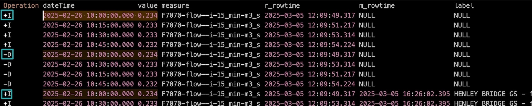
The magic button in the Flink shell is M - this shows the underlying changelog that the client is displaying. Note the highlights on the Operation column to see what’s happening:

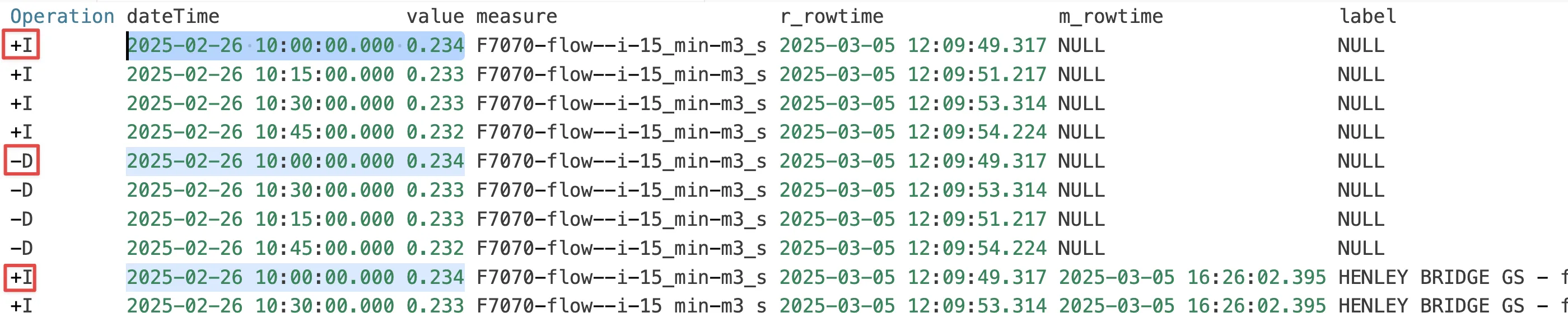
CleanShot%202025 03 05%20at%2017.06.02@2x

First up a row with no match is emitted (+I) from the join. After that a match is found, so the first result is retracted (-D) and replaced (the second +I). This happens for each of the four rows that we saw above.

Something else I saw in looking more closely at the rowtimes in the data was this:

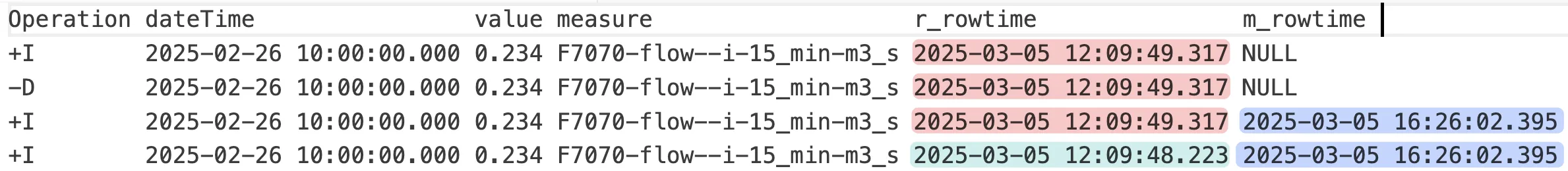
CleanShot%202025 03 05%20at%2017.21.33@2x

A seeming duplicate, after the initial retract & restatement with a successful join to measures, with a difference $ROWTIME on the readings table.

Let’s dig in even further and narrow it down to just this particular record:

SELECT r.`dateTime`,
	r.`value`, r.`measure`, r.`$rowtime` as r_rowtime, m.`$rowtime` as m_rowtime,
	m.`label`,
	m.`parameterName`
  FROM readings r
       LEFT OUTER JOIN `measures_with_pk` m
       ON r.`measure` = m.notation
 WHERE r.`measure` = 'F7070-flow--i-15_min-m3_s' AND r.dateTime = '2025-02-26 10:00:00.000';

Now it gets stranger…I don’t get the NULL at all—but I do get duplicates:

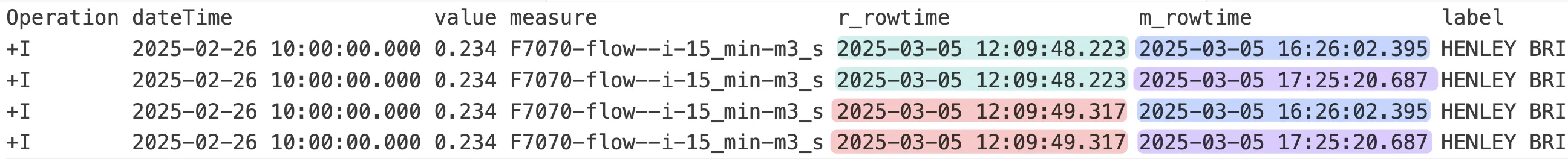
CleanShot%202025 03 05%20at%2017.34.29@2x 1

Where are the duplicates coming from? 🔗

So we’ve got two rows returned from readings ($ROWTIME of 12:09:48.223 and 12:09:49.317), and two from measures_with_pk ($ROWTIME of 17:25:20.687 and 16:26:02.395), giving us a cartesian result of four rows.

Looking at the measures data first, let’s confirm the presence of the duplicate, and then figure out what to do about it:

SELECT $rowtime, *
  FROM `measures_with_pk`
 WHERE notation='F7070-flow--i-15_min-m3_s';

$rowtime                notation                  datumType label
2025-03-05 16:26:02.395 F7070-flow--i-15_min-m3_s NULL      HENLEY BRIDGE GS - flow--i-15_min-m3_s
2025-03-05 17:25:20.687 F7070-flow--i-15_min-m3_s NULL      HENLEY BRIDGE GS - flow--i-15_min-m3_s

Checking the table definition again, I’ve maybe not got it quite right:

SHOW CREATE TABLE `measures_with_pk`;
[…]
  CREATE TABLE `default`.`cluster_0`.`measures_with_pk` (
    `notation` VARCHAR(2147483647) NOT NULL,
[…]
    CONSTRAINT `PK_notation` PRIMARY KEY (`notation`) NOT ENFORCED
  )
  DISTRIBUTED BY HASH(`notation`) INTO 6 BUCKETS
  WITH (
    'changelog.mode' = 'append',
    'kafka.cleanup-policy' = 'compact',
    'kafka.retention.size' = '0 bytes',
    'kafka.retention.time' = '7 d',
	[…]

The PK is defined, yes—but I think there are two problems here:

'kafka.retention.time' = '7 d': If there’s no new data pulled into the source topic (flood-monitoring-measures) for a week then the data will age out of this table, and we don’t want that (ref).
'changelog.mode' = 'append', (ref): as this is a dimension table, we don’t want to add (append) data to it, but update existing values for a key or insert them if they don’t exist—which is what upsert does.

Let’s try changing these.

-- See https://docs.confluent.io/cloud/current/flink/reference/sql-examples.html#table-with-infinite-retention-time
ALTER TABLE `measures_with_pk`
	SET ('changelog.mode' = 'upsert',
	     'kafka.retention.time' = '0');

Now when I query the table I get a single row returned. Note the $rowtime; it’s as of today (2025-03-07), since I took a break in writing this since running the query last (as seen on the $rowtime in the query output above, 2025-03-05)

$rowtime                notation                  datumType label                                  parameter
2025-03-07 10:47:17.385 F7070-flow--i-15_min-m3_s NULL      HENLEY BRIDGE GS - flow--i-15_min-m3_s flow

We can also confirm the underlying Kafka topic configuration is now correct:

$ confluent kafka topic configuration list measures_with_pk;
                   Name                   |        Value        | Read-Only
------------------------------------------+---------------------+------------
  cleanup.policy                          | compact             | false
[…]
  retention.bytes                         | -1                  | false
  retention.ms                            | -1                  | false

Going back to the join between readings and measures, let’s see how the data now looks:

dateTime                value measure                   r_rowtime               m_rowtime               label                                  parameterName
2025-02-26 10:00:00.000 0.234 F7070-flow--i-15_min-m3_s 2025-03-05 12:09:49.317 2025-03-07 10:47:17.385 HENLEY BRIDGE GS - flow--i-15_min-m3_s Flow
2025-02-26 10:00:00.000 0.234 F7070-flow--i-15_min-m3_s 2025-03-05 12:09:48.223 2025-03-07 10:47:17.385 HENLEY BRIDGE GS - flow--i-15_min-m3_s Flow

Still a duplicate entry for the measure at 2025-02-26 10:00:00.000, because of two entries in the readings table (note the different r_rowtime).

In the readings table we can see the duplicate (as you’d expect, based on the output above):

SELECT $rowtime, *
  FROM readings
 WHERE `measure` = 'F7070-flow--i-15_min-m3_s' AND `dateTime` = '2025-02-26 10:00:00.000';

$rowtime                publisher          version dateTime                measure                   value
2025-03-05 12:09:48.223 Environment Agency 0.9     2025-02-26 10:00:00.000 F7070-flow--i-15_min-m3_s 0.234
2025-03-05 12:09:49.317 Environment Agency 0.9     2025-02-26 10:00:00.000 F7070-flow--i-15_min-m3_s 0.234

One thing I want to check is that there’s a single process writing to the table—given that as we work our way through this exploration, there may be things lying around that we’ve not tidied up.

We can look at what statements are running using the statement list command and filter it with jq:

$ confluent flink statement list --output json | \
  jq '.[] | select((.statement | contains("readings")) and (.status == "RUNNING")) '

{
  "creation_date": "2025-03-03T15:35:35.945202Z",
  "name": "cli-2025-03-03-153534-4c63832d-187e-481c-9091-24f6147e226f",
  "statement": "CREATE TABLE readings AS\nSELECT meta.publisher, meta.version, i.dateTime, i.measure,i.`value` FROM `flood-monitoring-readings` r\n  CROSS JOIN UNNEST(r.items) AS i;",
  "compute_pool": "lfcp-kzky6g",
  "status": "RUNNING",
  "latest_offsets": null,
  "latest_offsets_timestamp": "0001-01-01T00:00:00Z"
}
{
  "creation_date": "2025-03-05T12:09:29.082467Z",
  "name": "cli-2025-03-05-120928-608894cd-4a72-473f-b80c-0a35ea6e41cc",
  "statement": "CREATE TABLE readings AS\nSELECT meta.publisher, \n   meta.version, \n   i.dateTime, \n   REGEXP_REPLACE(i.measure, \n  'http://environment\\.data\\.gov\\.uk/flood-monitoring/id/measures/', \n  '') AS measure,\n   i.`value` \n  FROM `flood
-monitoring-readings` r\n   CROSS JOIN UNNEST(r.items) AS i;",
  "compute_pool": "lfcp-kzky6g",
  "status": "RUNNING",
  "latest_offsets": null,
  "latest_offsets_timestamp": "0001-01-01T00:00:00Z"
}

So there are two statements running. However, this isn’t quite the smoking gun you’d think, because as you can see in the query output above (and in fact, in the WHERE clause too) the measure field is the newer version without the URL base prefix: F7070-flow—i-15_min-m3_s. The other query that’s running still is just selecting the unmodified measure column. That’s not to say that it’s not also creating duplicate/redundant data on the readings table, but it doesn’t account for the duplicate that we’re seeing.

Let’s remove the query, so that we have just the correct one running:

$ confluent flink statement delete cli-2025-03-03-153534-4c63832d-187e-481c-9091-24f6147e226f

Digging into the table some more there are plenty of rows where there is just one entry for a measure; but also a consistent pattern over time where there are duplicates:

SELECT dateTime, `measure`, COUNT(*) FROM readings WHERE `measure` = 'F7070-flow--i-15_min-m3_s'
 GROUP BY dateTime, `measure` ;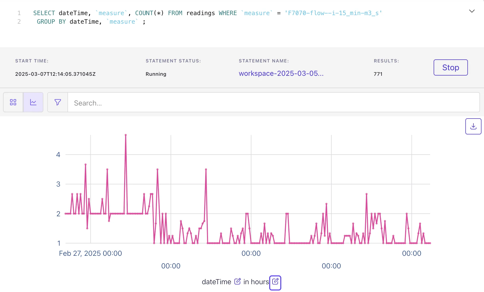

CleanShot%202025 03 07%20at%2012.25.16@2x

Why are there duplicates in `readings`? 🔗

Let’s go back to the source table for readings and see if there are duplicates in that—if it, as is more likely, in our futzing around with re-creating readings earlier we made a snafu and ran two queries at once.

This is the query that creates the readings table:

CREATE TABLE readings AS
	SELECT meta.publisher,
		   meta.version,
		   i.dateTime,
		   REGEXP_REPLACE(i.measure,
				  'http://environment\.data\.gov\.uk/flood-monitoring/id/measures/',
				  '') AS measure,
		   i.`value`
	  FROM `flood-monitoring-readings` r
		   CROSS JOIN UNNEST(r.items) AS i;

Let’s run just the SELECT, and add the predicate we used above, to see if we see the same duplicates.

WITH readings_cte AS
	(SELECT $rowtime,
			meta.publisher,
		   meta.version,
		   i.dateTime,
		   REGEXP_REPLACE(i.measure,
				  'http://environment\.data\.gov\.uk/flood-monitoring/id/measures/',
				  '') AS measure,
		   i.`value`
	  FROM `flood-monitoring-readings` r
		   CROSS JOIN UNNEST(r.items) AS i)
SELECT * FROM readings_cte
  WHERE `measure` = 'F7070-flow--i-15_min-m3_s';

Yep, still duplicates - with different $rowtime

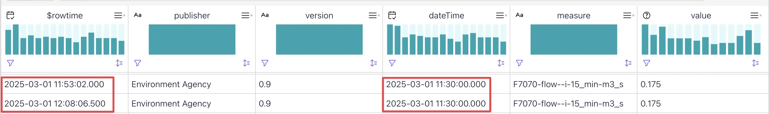
CleanShot%202025 03 07%20at%2014.35.45@2x

Going all the way back to the source, here are the messages on the Kafka topic:

$ kcat -b my-broker.aws.confluent.cloud:9092 \
        -X security.protocol=sasl_ssl -X sasl.mechanisms=PLAIN \
        -X sasl.username=$CC_API \
        -X sasl.password=$CC_SECRET \
        -s avro \
        -r https://$SR_API:$SR_SECRET$@my_sr.aws.confluent.cloud | jq '.items[] | select (.measure | contains("F7070"))' \
        -C -t flood-monitoring-readings -o s@$(date -d "2025-03-01 11:53:02.000" +%s%3N) -c2
{
  "_40id": "http://environment.data.gov.uk/flood-monitoring/data/readings/F7070-flow--i-15_min-m3_s/2025-03-01T11-30-00Z",
  "dateTime": 1740828600000,
  "measure": "http://environment.data.gov.uk/flood-monitoring/id/measures/F7070-flow--i-15_min-m3_s",
  "value": 0.17499999999999999
}
{
  "_40id": "http://environment.data.gov.uk/flood-monitoring/data/readings/F7070-flow--i-15_min-m3_s/2025-03-01T11-30-00Z",
  "dateTime": 1740828600000,
  "measure": "http://environment.data.gov.uk/flood-monitoring/id/measures/F7070-flow--i-15_min-m3_s",
  "value": 0.17499999999999999
}

Where does that leave us?

It suggests that readings of particular measures may sometimes lag being reported, and thus the API serves up the previous value. We also have the period field in measure which could vary, and not be the same as—nor in sync with—the frequency with which we’re polling the API to get the data.

So we need to change our readings table. Just like measures_with_pk needed defining correctly when it came to the changelog and retention, so the readings table (and stations_with_pk too, once we’re done here). Since we’re rebuilding it we’ll add in the headers too whilst we’re at it.

CREATE TABLE readings01 (
	`dateTime` TIMESTAMP(3) WITH LOCAL TIME ZONE NOT NULL,
	`measure` VARCHAR,
	`value` DOUBLE NOT NULL,
	headers MAP<VARCHAR(9) NOT NULL, STRING NOT NULL> METADATA,
	PRIMARY KEY (`dateTime`,`measure`) NOT ENFORCED)
	DISTRIBUTED BY HASH(`dateTime`,`measure`) INTO 6 BUCKETS
	WITH ('changelog.mode' = 'upsert',
	     'kafka.retention.time' = '0');

INSERT INTO readings01
  SELECT  i.dateTime,
		   REGEXP_REPLACE(i.measure,
				  'http://environment\.data\.gov\.uk/flood-monitoring/id/measures/',
				  '') AS measure,
		   i.`value`,
		   MAP['publisher',publisher,'version',version] AS headers
	  FROM `flood-monitoring-readings` r
		   CROSS JOIN UNNEST(r.items) AS i;

Let’s check the new readings01 table for the same measure and time period as we were examining above:

SELECT * FROM readings01
  WHERE measure = 'F7070-flow--i-15_min-m3_s'
    AND dateTime BETWEEN '2025-03-01 10:00:00.000' AND '2025-03-01 13:00:00.000';

dateTime                measure                   value headers
2025-03-01 10:00:00.000 F7070-flow--i-15_min-m3_s 0.177 {version=0.9, publisher=Environment Agency}
2025-03-01 10:15:00.000 F7070-flow--i-15_min-m3_s 0.177 {version=0.9, publisher=Environment Agency}
2025-03-01 10:45:00.000 F7070-flow--i-15_min-m3_s 0.177 {version=0.9, publisher=Environment Agency}
2025-03-01 11:00:00.000 F7070-flow--i-15_min-m3_s 0.177 {version=0.9, publisher=Environment Agency}
2025-03-01 11:30:00.000 F7070-flow--i-15_min-m3_s 0.175 {version=0.9, publisher=Environment Agency}
2025-03-01 12:00:00.000 F7070-flow--i-15_min-m3_s 0.175 {version=0.9, publisher=Environment Agency}
2025-03-01 12:15:00.000 F7070-flow--i-15_min-m3_s 0.175 {version=0.9, publisher=Environment Agency}
2025-03-01 12:45:00.000 F7070-flow--i-15_min-m3_s 0.174 {version=0.9, publisher=Environment Agency}
2025-03-01 13:00:00.000 F7070-flow--i-15_min-m3_s 0.174 {version=0.9, publisher=Environment Agency}

(I manually sorted the lines chronologically to make it easier to examine).

Now we have just one reading stored for dateTime=2025-03-01 11:30:00.000. Looking at the changelog you can see the duplicate coming in and replacing what was there already for that time:

Operation dateTime                measure                   value headers
[…]
+I        2025-03-01 11:30:00.000 F7070-flow--i-15_min-m3_s 0.175 {version=0.9, publisher=Environment Agency}
-U        2025-03-01 11:30:00.000 F7070-flow--i-15_min-m3_s 0.175 {version=0.9, publisher=Environment Agency}
+U        2025-03-01 11:30:00.000 F7070-flow--i-15_min-m3_s 0.175 {version=0.9, publisher=Environment Agency}
[…]

Let’s try the join again 🔗

Phew. That was quite the detour. Now that we’ve changed the types of the tables to upsert and defined a primary key for each, we should hopefully get no duplicates when we run this query against the new readings01 table:

SELECT r.`dateTime`,
	   r.`value`,
	   r.`measure`,
	   r.`$rowtime` as r_rowtime,
	   m.`$rowtime` as m_rowtime,
	   m.`label`,
	   m.`parameterName`
  FROM readings01 r
       LEFT OUTER JOIN `measures_with_pk` m
       ON r.`measure` = m.notation
 WHERE r.`measure` = 'F7070-flow--i-15_min-m3_s' AND r.dateTime = '2025-02-26 10:00:00.000';

The results look good. We can directly check for duplicates too:

SELECT dateTime, `measure`, COUNT(*) FROM readings01 WHERE `measure` = 'F7070-flow--i-15_min-m3_s'
 GROUP BY dateTime, `measure` ;

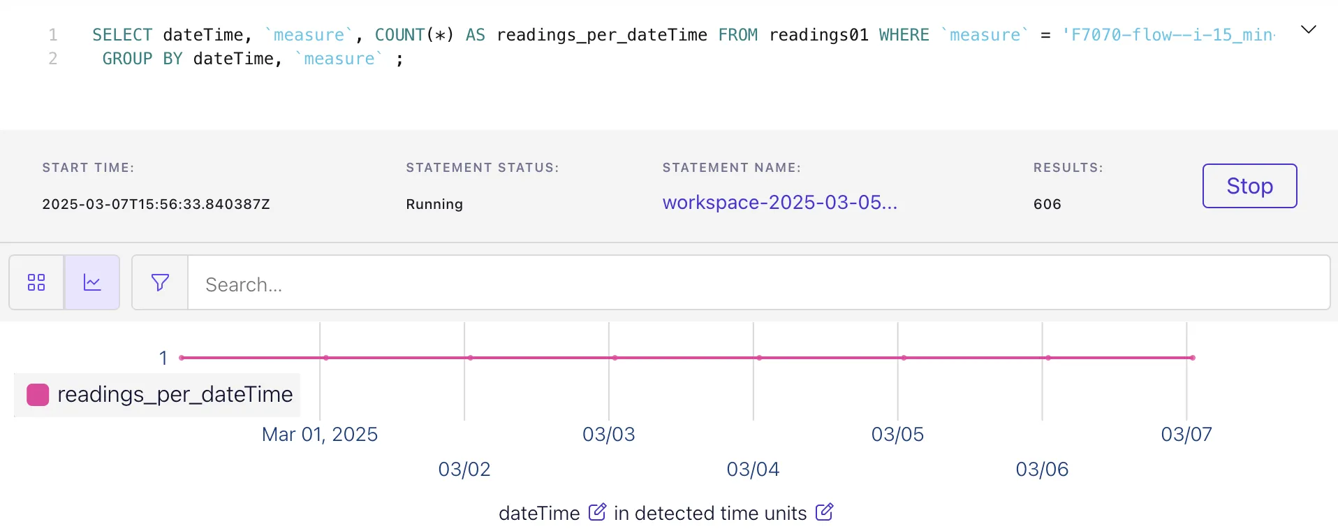
Huzzah!

Joining the data to `stations` 🔗

We’ll learn from what we did above, and update stations with the correct changelog and retention settings:

ALTER TABLE `stations_with_pk`
	SET ('changelog.mode' = 'upsert',
	     'kafka.retention.time' = '0');

Now we’ll try a join across all three entities - for a given reading, enrich it with measure details and station details.

SELECT  r.`dateTime`,
	r.`value`,
	m.`parameterName`,
	m.`unitName`,
	s.`label`,
	s.`town`,
	s.`riverName`,
	s.`catchmentName`,
	m.`label`,
	m.`period`,
	m.`qualifier`,
	m.`valueType`,
	s.`stationReference`,
	s.`dateOpened`,
	s.`easting`,
	s.`northing`,
	s.`lat`,
	s.`long`
  FROM readings01 r
       LEFT OUTER JOIN `measures_with_pk` m
       ON r.`measure` = m.notation
       LEFT OUTER JOIN `stations_with_pk` s
       ON m.stationReference = s.stationReference;

and…it works!

Let’s take a look at a specific station:

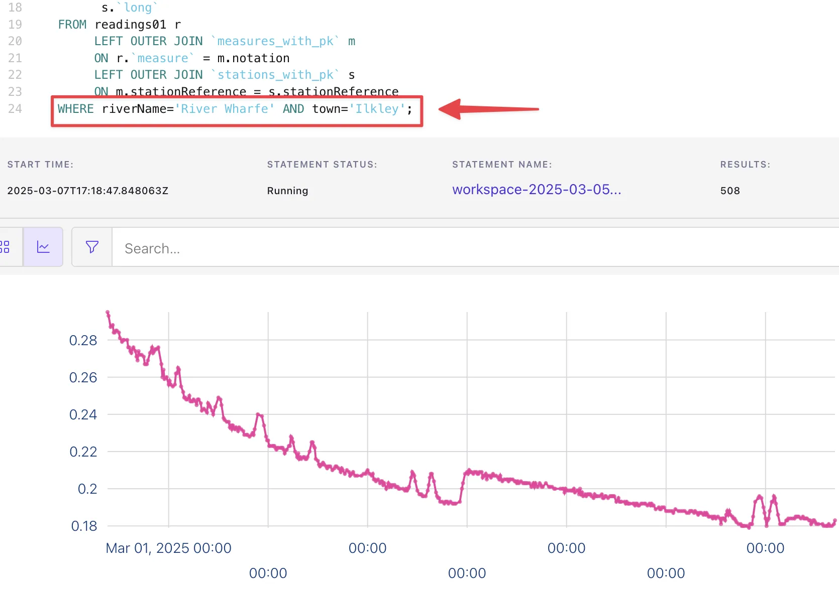
CleanShot%202025 03 07%20at%2017.29.32@2x

That was fun :) Stay tuned for more Flink-y fun and data wrangling!

💡 I built this blog using Apache Flink for Confluent Cloud which is why you see things like the nice data visualisations and automatic table/topic mappings.

AFAIK the principles should all be the same if you want to use Apache Flink too; the CLI is slightly different, and you’ll have to figure out your own dataviz :)

The Plan 🔗

Writing Kafka headers from Flink SQL 🔗

Handling dimensions in Flink SQL 🔗

Setting the Kafka record key 🔗

Changing the Kafka topic under a Flink table to compacted 🔗

Changing the key 🔗

Changing the foreign key (FK) on readings 🔗

Sidebar: How many times are there? 🔗

Joining Kafka topics in Flink SQL 🔗

Where are the duplicates coming from? 🔗

Why are there duplicates in readings? 🔗

Let’s try the join again 🔗

Joining the data to stations 🔗

Changing the foreign key (FK) on `readings` 🔗

Why are there duplicates in `readings`? 🔗

Joining the data to `stations` 🔗